“Nothing is certain except for death and taxes.”
This isn’t a dataset made with a bed of roses or manicured green grass. A bit more serious. Let’s see if we can quickly learn anything here. The dataset is the following.
“name” : “NCHS – Leading Causes of Death: United States”,
“attribution” : “National Center for Health Statistics”,
The public dataset is available at https://data.cdc.gov/api/views/bi63-dtpu/rows.json?accessType=DOWNLOAD
Step 1: Download the file into a local file (e.g. health.json). Upload this file to one of the nodes in the Couchbase cluster.
Step 2: import the data into a bucket called cause. After you create the bucket, create the primary index. You’ll need this for querying.
/opt/couchbase/bin/cbimport json -c couchbase://127.0.0.1 -u Administrator -p password -b cause -d file://health.json -g cause:0 -f sample
> CREATE PRIMARY INDEX ON cause;
Step 3. Inspect the structure of the data.
All of the data is provided in a SINGLE JSON document. Because of this, INFER doesn’t help. You’ll have to inspect and understand the structure manually. This data in typical government dataset with a lot of data in simple arrays with the meaning of each entity given at in the metadata.
Simple array:
|
1 |
<strong>select data from cause ;</strong> |
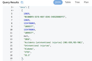
This simply contains an array of data without the schema. For the public datasets, the schema is in the meta field.
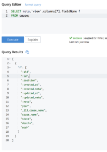
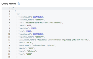
Let’s transform the structure into simple JSON key-value pairs so we can handle these bit more effectively. You can learn more about how this magic happened in this article.
|
1 2 3 4 5 6 7 8 9 10 11 12 13 14 15 16 |
WITH cs AS ( SELECT meta.`view`.columns [*].fieldName f, data FROM cause ) SELECT o FROM cs UNNEST cs.data AS d1 LET o = OBJECT p :d1 [ARRAY_POSITION(cs.f, p)] FOR p IN cs.f END; |
Task1: Find out the cause for most deaths in a state, by year.
The common table expression (CTE) in the WITH clause (csdata) transforms the complex json data into flat JSON. You can do this dynamically or do this once and INSERT back into a bucket, as I’ve discussed in the article on New York baby names. In this article, I use CTEs.
|
1 2 3 4 5 6 7 8 9 10 11 12 13 14 15 16 17 18 19 20 21 22 23 24 25 26 27 28 29 30 31 32 |
WITH csdata as ( WITH cs AS ( SELECT meta.`view`.columns [*].fieldName f, data FROM cause ) SELECT o FROM cs UNNEST cs.data AS d1 LET o = OBJECT p :d1 [ARRAY_POSITION(cs.f, p)] FOR p IN cs.f END ) SELECT c.o.state, c.o.year, c.o.cause_name, COUNT(c.o.cause_name), SUM(TONUMBER(c.o.deaths)) totdeaths FROM csdata as c WHERE c.o.state <> "United States" and c.o.cause_name <> "All causes" GROUP BY c.o.state, c.o.year, c.o.cause_name ORDER BY totdeaths DESC, c.o.state, c.o.year |
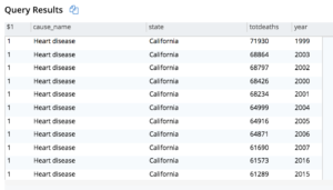
In this case, all the deaths in California come on top, mainly due to its population.
Task 2. Find out leading causes of death in each state for the year 2016.
Query 2: Use the resultset from the previous query and then use the FIRST_VALUE() window function to determine the top cause. Partitioning by state (in the OVER BY clause) will give you the partitions by state and ORDER BY dx.totdeaths within the OVER BY clause will give you the top cause in every state.
|
1 2 3 4 5 6 7 8 9 10 11 12 13 14 15 16 17 18 19 20 21 22 23 24 25 26 27 28 29 30 31 32 33 34 35 36 37 38 |
WITH csdata as ( WITH cs AS ( SELECT meta.`view`.columns [*].fieldName f, data FROM cause ) SELECT o FROM cs UNNEST cs.data AS d1 LET o = OBJECT p :d1 [ARRAY_POSITION(cs.f, p)] FOR p IN cs.f END ), d2 as( SELECT c.o.state, c.o.year, c.o.cause_name, SUM(TONUMBER(c.o.deaths)) totdeaths FROM csdata as c WHERE c.o.state <> "United States" and c.o.cause_name <> "All causes" and c.o.year = "2016" GROUP BY c.o.state, c.o.year, c.o.cause_name), d3 as ( SELECT dx.state, dx.cause_name, dx.totdeaths, FIRST_VALUE(dx.cause_name) OVER(PARTITION BY dx.state ORDER BY dx.totdeaths DESC) topreason, FIRST_VALUE(dx.totdeaths) OVER(PARTITION BY dx.state ORDER BY dx.totdeaths DESC) topcount FROM d2 dx) SELECT d3 FROM d3 WHERE d3.topcount = d3.totdeaths order by d3.state |
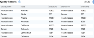

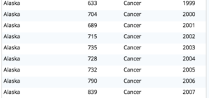
Task 3. Find out how the top reason has changed by the year, from 1999 to 2016 by state.
Query 3: Simply generate the report for all the years (199-2016) and then determine the top reason and finally get the highest reason by grouping by state, year and getting MAX(topcount) for the topreason cause.
|
1 2 3 4 5 6 7 8 9 10 11 12 13 14 15 16 17 18 19 20 21 22 23 24 25 26 27 28 29 30 31 32 33 34 35 36 37 |
WITH csdata as ( WITH cs AS ( SELECT meta.`view`.columns [*].fieldName f, data FROM cause ) SELECT o FROM cs UNNEST cs.data AS d1 LET o = OBJECT p :d1 [ARRAY_POSITION(cs.f, p)] FOR p IN cs.f END ), d2 as( SELECT c.o.state, c.o.year, c.o.cause_name, SUM(TONUMBER(c.o.deaths)) totdeaths FROM csdata as c WHERE c.o.state <> "United States" and c.o.cause_name <> "All causes" GROUP BY c.o.state, c.o.year, c.o.cause_name), d3 as ( SELECT dx.state, dx.year, FIRST_VALUE(dx.cause_name) OVER(PARTITION BY dx.state, dx.year ORDER BY dx.totdeaths DESC ) topreason, FIRST_VALUE(dx.totdeaths) OVER(PARTITION BY dx.state, dx.year ORDER BY dx.totdeaths DESC) topcount FROM d2 dx) SELECT d3.state , d3.year , d3.topreason, max(d3.topcount) topcount FROM d3 GROUP BY d3.state, d3.year, d3.topreason order by d3.state, d3.year |
Here’s the partial result.
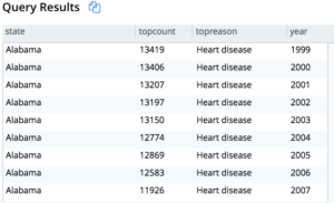
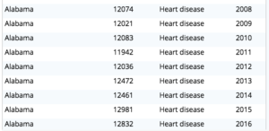
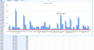
Visualizing this gives us the following histogram.
