Semantic Similarity with Focused Selectivity

Why does semantic search need selectivity?

Up until now, we’ve viewed a vector embedding as a complete, stand-alone entity – focused entirely on the meaning it encodes. While this enables semantic search, often with a high degree of similarity, it remains limited to similarity among the query and dataset embeddings.

The vector similarity search offering could not be relied upon to satisfy exact predicates. Pre-filtering aims to address exactly this gap – by searching for similar vectors only among those satisfying some filtering criteria.

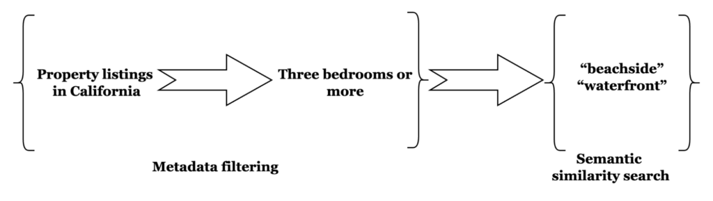
It’s the embedding equivalent of limiting your search, whether for a job or a property, to a location. Say, you want a beachfront property in a specific state. You also want to limit your search to those with three bedrooms or more. Combing through listings without a method to filter for these criteria is almost unfeasible given a lot of listings.

With pre-filtering, you can limit your search to a specific location by restricting the search space to eligible properties via geospatial and numeric queries. A vector similarity search for “beach-front”, “beachside”, “waterfront” properties will be performed over this limited subset.

Pre-filtering will allow users to specify filter queries as part of the kNN attribute in the query, only the results of which will be considered as eligible to be returned by the kNN query. Simply put, the user can now use the familiar FTS query syntax to restrict the documents over which a kNN search will be performed.

When to apply pre-filtering?

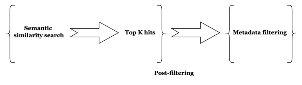
As the name suggests, the embeddings are metadata-filtered before the similarity search. This is different from post-filtering where a kNN search is followed by metadata-filtering. Pre-filtering offers a much higher chance of returning k hits, assuming there are at least those many documents which pass the filtering stage.

How this works

Before we get into the guts of pre-filtering with kNN, let’s understand how a vector and full-text index are co-located in the Search service index. Each Search index has one or more partitions, each of which has one or more segments. Each of these segments is a file, and the file is divided into separate sections, with one per type of index. Viewing a segment as a self-contained unit with both text and vector content of a batch of documents indexed will be useful for understanding how pre-filtering works at the segment level.

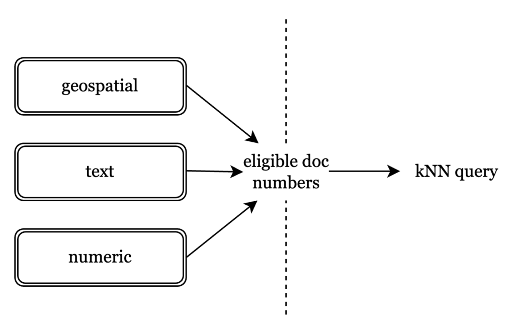A key consideration when building this was that it should be predicate-agnostic at search time. Essentially, this means that the filtering at the vector index should work the same way, irrespective of the full-text predicate. A text predicate over a text field should be no different from a numerical predicate over another.

To this end, document numbers, identifiers unique to a document, are used to demarcate which documents are eligible for the kNN query. Every FTS query, whether text, numeric, or geospatial, boils down to identifying hits by their document number. Using document numbers means we do not have to change our indexing strategy for vectors, and limit it to a search time change.

Phase 1: Metadata filtering

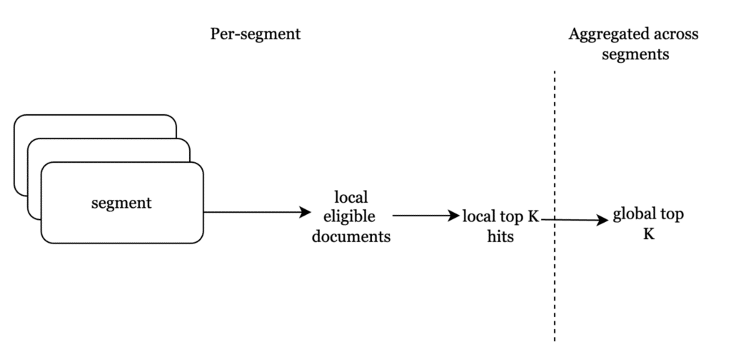
Since a segment is essentially an immutable batch of documents, with their text and vector content indexed, the full-text metadata query returns all eligible documents at the segment level. Their document numbers are then passed to the vector index to retrieve the nearest eligible vectors.

Phase 2: kNN search

The current algorithm which picks the nprobe clusters closest to the query vector in an IVF index is essentially flying blind since it does not account for proximate clusters with few to no eligible documents. At search time, the selection of clusters to probe now has to account for distribution of metadata-filtered hits across the index.

A cluster closer to the query vector might have far fewer eligible hits than one much farther.

Taking into account filter hit distribution while keeping recall high means that we cannot scan clusters solely on the basis of filter hit density. What it does mean is that we attempt to minimize distance computations for ineligible vectors, even as we scan as many clusters as needed to return the k nearest neighbors.

Earlier, nprobe was defined as the absolute limit to the number of clusters scanned. Now, it’s more of a minimum number of clusters to scan assuming fewer clusters have enough eligible vectors. In cases of sparse filter hit distribution, where each cluster has relatively few eligible vectors, our quest for k nearest neighbours can lead us to scan far more than nprobe clusters. Both filtered and unfiltered kNN scan clusters in increasing order of distance from the query vector, with the difference lying in scanning a subset of vectors across a potentially larger number of clusters.

Once the vector index returns the most similar vectors at a segment level, these are aggregated at a global index level similar to how it’s done for kNN without filtering.

How to use this

Let’s take a bucket, landmarks. This is a sample document:

Create an index, test, which indexes the embedding, id and city fields.

My first query is an embedding of the Royal Engineers Museum in Gillingham:

The closest hits I get are the London Fire Brigade Museum, the Verulamium Museum in St Albans and the RAF Museum in London.

We now want to search for similar museums in Glasgow, that is, the city field should have a value Glasgow.

Here’s how the filtered query looks, with the filter clause added:

As expected, the results are now limited to those in Glasgow – the closest being the Kelvingrove Art Gallery and Museum and the Riverside Museum.

As seen in this example, a filtered kNN query offers the advantage of selecting the documents for a similarity search using good, ol’ FTS queries.

Keep learning

• • Read blog to learn more about FAISS and vector indexing, Vector Search Performance: The Rise of Recall
  • Build LLM Apps That Are Faster and Cheaper With Couchbase
  • What is Semantic Search?
  • Start using Couchbase Capella today, for free