Autores y equipo de ingeniería: Bingjie Miao, Keshav Murthy, Marco Greco, Prathibha Bisarahalli. Couchbase, Inc.
Un optimizador basado en reglas conoce reglas para todo y costes para nada - Oscar Wilde
Resumen
Couchbase es una base de datos JSON distribuida. Proporciona procesamiento de datos distribuido, indexación de alto rendimiento y lenguaje de consulta declarativo N1QL junto con índice de búsqueda, eventos y análisis. N1QL (Non First Normal Query Language) es SQL para JSON. N1QL es a JSON lo que SQL es a las relaciones. Los desarrolladores dicen lo que hay que hacer y el motor N1QL resuelve el "cómo". El optimizador actual de N1QL es un optimizador basado en reglas. Cost Based Optimizer(CBO) para SQL fue inventado en IBM hace unos 40 años y ha sido fundamental para el éxito de los RDBMS y la productividad del desarrollador/DBA. Las bases de datos NoSQL se inventaron hace unos 10 años. Poco después de su invención, las bases de datos NoSQL empezaron a añadir un lenguaje de consulta similar a SQL con rutas de acceso limitadas y capacidades de optimización. La mayoría utilizan optimizadores basados en reglas o simplemente admiten la optimización basada en costes sólo para valores escalares simples (cadenas, números, booleanos, etc.).
Para crear un CBO sobre el modelo JSON, primero hay que recopilar y organizar las estadísticas. ¿Cómo recopilar, almacenar y utilizar estadísticas sobre el esquema flexible de JSON? ¿Cómo recopilar estadísticas sobre objetos, matrices y elementos dentro de objetos? ¿Cómo utilizarlas eficazmente en el optimizador?
Lukas Eder me dijo una vez: "El optimizador basado en costes hace que SQL sea totalmente declarativo". Tiene razón. Couchbase 6.5 (ahora GA) tiene Optimizador Basado en Costos para N1QL. Este artículo presenta la introducción de N1QL Cost Based Optimizer (CBO) en Couchbase 6.5. CBO es una función pendiente de patente. En este artículo describimos cómo utilizar CBO y los detalles de su implementación.
La versión PDF de este artículo está disponible en descargar aquí.
Índice
- Resumen
- Introducción a N1QL
- Optimizador basado en costes para N1QL
- Optimizador N1QL
- Optimizador basado en costes para N1QL
- Recogida de estadísticas para N1QL CBO
- Resumen
- Recursos Optimizador basado en reglas N1QL
- Referencias
Introducción a N1QL
Como JSON ha sido cada vez más aceptado por la industria de la tecnología de la información como lingua franca para el cambio de información, ha habido un aumento exponencial en la necesidad de repositorios que almacenen, actualicen y consulten documentos JSON de forma nativa. SQL ha añadido funciones que manipulan JSON en SQL:2016. SQL:2016 añade nuevas funciones escalares y de tabla para manipular JSON. Un enfoque alternativo es tratar JSON como el modelo de datos y diseñar el lenguaje para operar en JSON de forma nativa. N1QL y SQL utilizan este último enfoque y proporcionan un acceso natural a escalares, objetos, matrices, matrices de objetos, matrices dentro de objetos, etc.
|
1 2 3 4 5 6 7 8 9 10 11 12 13 14 15 16 |
SQL:2016: En: Microsoft SQL Servidor. SELECCIONE Nombre, Apellido, JSON_VALUE(jsonCol,$.info.dirección.CódigoPostal) AS Código postal, JSON_VALUE(jsonCol,'$.info.address. "Dirección Línea 1"')+' ' +JSON_VALUE(jsonCol,'$.info.address. "Dirección Línea 2"') AS Dirección, JSON_QUERY(jsonCol,$.info.skills) AS Habilidades DESDE Personas DONDE ISJSON(jsonCol) > 0 Y JSON_VALUE(jsonCol,'$.info.direccion.Ciudad')=Belgrado Y Estado=Activo ORDENAR POR JSON_VALUE(jsonCol,$.info.dirección.CódigoPostal) |
|
1 2 3 4 5 6 7 8 9 10 |
N1QL: Mismo consulta escrito en N1QL en el JSON modelo SELECCIONE Nombre, Apellido, jsonCol.info.address.PostCode AS Código postal, (jsonCol.info.address.`Dirección Línea 1` + ' ' + jsonCol.`info.address.`Dirección Línea 2`) AS Dirección, jsonCol.info.habilidades' Habilidades AS DE Personas DONDE jsonCol.info.address.Town = 'Belgrado' AND Estado='Activo ORDENAR POR jsonCol.info.address.PostCode |
Aprenda N1QL en https://query-tutorial.couchbase.com/
Servidor Couchbase:
Couchbase tiene motores que soportan N1QL:
- N1QL para aplicaciones interactivas en el servicio de consulta.
- N1QL for Analytics en el servicio Analytics.
En este artículo, nos centramos en N1QL for Query (aplicaciones interactivas) implementado en el servicio de consultas. Todos los datos manipulados por N1QL se guardan en JSON dentro del almacén de datos Couchbase gestionado por el servicio de datos.
Para soportar el procesamiento de consultas sobre JSON, N1QL amplía el lenguaje SQL de muchas maneras:
-
- Soporte para esquemas flexibles en JSON semiestructurado autodescriptivo.
- acceder y manipular elementos en JSON: valores escalares, objetos, matrices, objetos de valores escalares, matrices de valores escalares, matrices de objetos, matrices de matrices, etc.
- Introducir un nuevo valor booleano, MISSING para representar un par clave-valor que falta en un documento, esto es distinto de un valor nulo conocido. Esto amplía la función lógica de tres valores a lógica de cuatro valores.
- Nuevas operaciones NEST y UNNEST para crear matrices y aplanar matrices, respectivamente.
- Ampliar las operaciones JOIN para trabajar con escalares, objetos y matrices JSON.
- Para acelerar el procesamiento de estos documentos JSON, los índices secundarios globales pueden crearse sobre uno o más valores escalares, valores escalares de matrices, objetos anidados, matrices anidadas, objetos, objetos de matrices, elementos de matrices.
- Añadir la capacidad de búsqueda integrada utilizando el índice de búsqueda invertido.
Uso de CBO para N1QL
Hemos introducido (CBO) en Couchbase 6.5 (ahora GA). Vamos a ver cómo utilizar la función antes de profundizar en los detalles.
- CREAR un nuevo cubo y cargar los datos del cubo de muestra viaje-muestra.
|
1 2 3 4 5 6 7 8 9 |
INSERTAR EN hotel(CLAVE id, VALOR h) SELECCIONE META().id id, h DESDE Viajar-muestra h DONDE tipo = "hotel" |
- Modelo de documento hotelero
He aquí un ejemplo de documento hotelero. Estos valores son escalares, objetos y matrices. Una consulta accederá a todos estos campos y los procesará.
|
1 2 3 4 5 6 7 8 9 10 11 12 13 14 15 16 17 18 19 20 21 22 23 24 25 26 27 28 29 30 31 32 33 34 35 36 37 38 39 40 41 42 43 44 45 46 47 48 49 50 51 52 53 54 55 56 57 58 59 60 61 62 63 64 65 66 67 68 69 70 71 72 73 74 75 76 77 |
{ "hotel": { "dirección": "Capstone Road, ME7 3JE", "alias": null, "checkin": null, "checkout": null, "ciudad": "Medway", "país": "Reino Unido", "descripción": "Albergue de verano de 40 camas a unos 5 km de Gillingham, ubicado en una intrincada Oast House reconvertida en un entorno semirural"., "direcciones": null, "email": null, "fax": null, "desayuno_gratuito": verdadero, "free_internet": falso, "free_parking": verdadero, "geo": { "exactitud": "RANGO_INTERPOLADO", "lat": 51.35785, "lon": 0.55818 }, "id": 10025, "nombre": "Albergue Juvenil Medway", "pets_ok": verdadero, "teléfono": "+44 870 770 5964", "precio": null, "public_likes": [ "Julius Tromp I", "Corrine Hilll", "Jaeden McKenzie", "Vallie Ryan", "Brian Kilback", "Lilian McLaughlin", "Sra. Moses Feeney", "Elnora Trantow" ], "revisiones": [ { "autor": "Ozella Sipes", "contenido": "Este fue nuestro segundo viaje aquí y lo disfrutamos tanto o más que el año pasado. Excelente ubicación frente al mercado francés y justo enfrente de la parada del tranvía. Muy conveniente para varios restaurantes pequeños pero buenos. Muy limpio y bien mantenido. El servicio de limpieza y el resto del personal son amables y serviciales. Disfrutamos mucho sentados en la terraza del 2º piso sobre la entrada y "mirando a la gente" en la avenida Esplanade, también hablando con nuestros compañeros. Algunos muebles podrían necesitar un poco de actualización o sustitución, pero nada importante.", "fecha": "2013-06-22 18:33:50 +0300", "ratings": { "Limpieza": 5, "Localización": 4, "En general": 4, "Habitaciones": 3, "Servicio": 5, "Valor": 4 } }, { "autor": "Barton Marks", "contenido": "Encontramos el hotel de la Monnaie a través de Interval y pensamos en darle una oportunidad mientras asistíamos a una conferencia en Nueva Orleans. Este lugar tenía una ubicación perfecta y sin duda era mejor que alojarse en el centro en el Hilton con el resto de los asistentes. Estábamos justo en el borde del Barrio Francés coning distancia a pie de toda la zona. La ubicación en Esplanade es más de una zona residencial por lo que está cerca de la diversión, pero lo suficientemente lejos para disfrutar de un tiempo de inactividad tranquila. Nos encantó el tranvía justo enfrente y lo cogimos hasta el centro de conferencias para los días de conferencias a los que asistimos. También lo cogimos hasta Canal Street y casi lo entregamos en el museo de la Segunda Guerra Mundial. Desde allí pudimos coger un tranvía hasta el Garden District, una visita obligada si te gusta la arquitectura antigua: preciosas casas antiguas (mansiones). Almorzamos en Joey K's y fue excelente. Comimos en tantos sitios en el Barrio Francés que no recuerdo todos los nombres. A mi marido le encantaron todas las comidas de NOL - gumbo, jambalya y más. Me alegro de haber encontrado Louisiana Pizza Kitchen justo al otro lado de la Casa de la Moneda (enfrente de Monnaie). Es un sitio pequeño, pero la pizza es excelente. El día que llegamos había un gran festival de jazz al otro lado de la calle. Sin embargo, una vez en nuestras habitaciones, no se oía ningún ruido exterior. Sólo el silbato del tren por la noche. Nos gustó estar tan cerca del Mercado Francés y a poca distancia de todos los sitios que ver. Y no se puede pasar por alto el Cafe du Monde en la calle - un lugar muy concurrido happenning con los mejores dougnuts francés!!!Delicioso! Sin duda volveremos y nos alojaríamos aquí de nuevo. No nos acosaron para que compráramos nada. Mi marido sólo recibió una llamada telefónica con respecto a tiempo compartido y la mujer era muy agradable. El personal era tranquilo y amable. Mi única queja fue la cama muy firme. Aparte de eso, disfrutamos mucho de nuestra estancia. Gracias Hotel de la Monnaie"., "fecha": "2015-03-02 19:56:13 +0300", "ratings": { "Servicio a empresas (por ejemplo, acceso a Internet)": 4, "Check in / recepción": 4, "Limpieza": 4, "Localización": 4, "En general": 4, "Habitaciones": 3, "Servicio": 3, "Valor": 5 } } ], "estado": null, "título: "Gillingham (Kent)", "tollfree": null, "tipo": "hotel", "url": "http://www.yha.org.uk", "vacante": verdadero } } |
- Una vez que conozca las consultas que desea ejecutar, sólo tiene que crear los índices con las claves.
|
1 2 3 4 5 6 7 8 9 10 11 |
CREAR ÍNDICE i3 EN `hotel`(nombre, país); CREAR ÍNDICE i4 EN `hotel`(país, nombre); CREAR ÍNDICE i3 EN `hotel`(país, ciudad); CREAR ÍNDICE i4 EN `hotel`(ciudad, país); /* Índices de matriz sobre las claves de matriz que desea filtrar. CREATE INDEX i5 ON `hotel`(DISTINCT public_likes); CREATE INDEX i6 ON `hotel`(DISTINCT ARRAY r.ratings.Overall FOR r IN reviews END); /* Índice de los campos del objeto geográfico */ CREAR ÍNDICE i7 EN `hotel`(geo.lat, geo.lon) |
- Ahora, recopile estadísticas sobre el campo en el que tendrá filtros. Típicamente, usted indexa los campos sobre los que indexa. Por lo tanto, también querrá recopilar estadísticas sobre ellos. A diferencia de la sentencia CREATE INDEX, el orden de las claves no tiene consecuencias para la sentencia UPDATE STASTICS
ACTUALIZACIÓN ESTADÍSTICAS para `hotel` (tipo, dirección, ciudad, país, free_breakfast, id, teléfono);
- Índice de matriz en una matriz simple de escalares. public_likes es una matriz de cadenas. DISTINCT gustos_públicos crea un índice en cada elemento de gustos_públicos en lugar de en toda la matriz gustos_públicos. Detalles de las estadísticas de array más adelante en el artículo.
ACTUALIZACIÓN ESTADÍSTICAS para `hotel`(DISTINTO public_likes);
- Ahora ejecute, explique y observe estas afirmaciones. El CBO, basándose en las estadísticas que recopiló anteriormente, calculó la selectividad para el predicado (país = "Francia")
|
1 2 3 4 |
SELECCIONAR recuento(*) DESDE `hotel` DONDE país = Francia; { "$1": 140 } |
- Aquí está el fragmento de EXPLAIN. La salida de Explain tendrá estimaciones de cardinalidad y la salida de profile tendrá los documentos reales (filas, claves) calificados en cada operador.
|
1 2 3 4 5 6 7 8 9 10 11 12 13 14 15 16 17 18 19 20 21 22 23 24 |
"#operator": "IndexScan3", "cardinalidad": 141.54221635883903, "coste": 71.19573482849603, "tapas": [ "cover ((`hotel`.`country`))", "cover ((`hotel`.`type`))", "cover ((meta(`hotel`).`id`))", "cover (count(*))" ], "índice": "i2", SELECCIONE cuente(*) DESDE `hotel` DONDE país = Estados Unidos; { "$1": 361 } "cardinalidad": 361.7189973614776, "coste": 181.94465567282322, "tapas": [ "cover ((`hotel`.`country`))", "cover ((`hotel`.`type`))", "cover ((meta(`hotel`).`id`))", "cover (count(*))" ], "índice": "i2", |
- combinando el cálculo de costes en predicados múltiples. Observe que los resultados reales son proporcionales a las estimaciones de cardinalidad. Unir estimaciones de selectividad son difíciles de estimar debido a las correlaciones y requieren técnicas adicionales.
|
1 2 3 4 5 6 7 8 9 10 11 12 13 14 15 16 17 18 19 20 21 22 23 24 25 26 27 28 29 30 31 32 33 34 35 36 37 38 39 40 41 42 43 44 |
SELECCIONE cuente(*) DESDE `hotel` DONDE país = Estados Unidos y nombre COMO A%; { "$1": 7 } "cardinalidad": 13.397476328354337, "coste": 8.748552042415382, "tapas": [ "cover ((`hotel`.`country`))", "portada ((`hotel`.`nombre`))", "cover ((meta(`hotel`).`id`))", "cover (count(*))" ], "índice": "i4", SELECCIONE cuente(*) DESDE `hotel` DONDE país = Estados Unidos y nombre = Ace Hotel DTLA { "$1": 1 } "#operator": "IndexScan3", "cardinalidad": 0.39466325234388644, "coste": 0.25771510378055784, "tapas": [ "portada ((`hotel`.`nombre`))", "cover ((`hotel`.`country`))", "cover ((meta(`hotel`).`id`))", "cover (count(*))" ], "índice": "i3", seleccione cuente(1) de hotel donde país = Estados Unidos y ciudad = San Francisco; { "$1": 132 } "#operator": "IndexScan3", "cardinalidad": 361.7189973614776, "coste": 181.94465567282322, "índice": "i2", "index_id": "a020ba7594f7c045", "proyección_índice": { "clave_primaria": verdadero }, "espacio clave": "hotel", |
- Cálculo sobre predicado de array: ANY. Esto utiliza la colección de estadísticas de la expresión (DISTINCT public_likes) en las estadísticas UPDATE anteriores. Las estadísticas de matrices son diferentes de las estadísticas escalares normales del mismo modo que las claves de índice de matrices son diferentes de las claves de índice normales. El histograma de public_keys contendrá más de un valor del mismo documento. Por lo tanto, todos los cálculos tendrán que tenerlo en cuenta para que las estimaciones se acerquen más a la realidad.
|
1 2 3 4 5 6 7 8 9 10 11 12 13 14 15 16 17 18 19 20 21 |
SELECCIONE CONTAR(1) DESDE hotel DONDE CUALQUIER p EN me gusta_público SATISFACE p COMO A% FIN { "$1": 272 } "#operator": "DistinctScan", "cardinalidad": 151.68407386905272, "coste": 144.52983565532256, "escanear": { "#operator": "IndexScan3", "cardinalidad": 331.49044875073974, "coste": 143.53536430907033, "tapas": [ "cover ((distinct ((`hotel`.`public_likes`))))", "cover ((meta(`hotel`).`id`))" ], |
- Cálculo sobre predicado de array sobre un campo dentro de un objeto de un array: ANY r IN reviews SATISFIES r.ratings.Overall = 4 END. Las estadísticas se recopilan en la expresión: (DISTINCT ARRAY r.ratings.Overall FOR r IN reviews END). La expresión de recopilación de estadísticas debe ser exactamente la misma que la expresión de matriz de clave de índice.
|
1 2 3 4 5 6 7 8 9 10 11 12 13 14 15 16 17 18 19 20 21 22 23 24 25 26 27 28 29 30 31 32 33 34 35 36 37 38 39 40 41 42 43 44 45 46 47 |
SELECCIONE CONTAR(1) DESDE hotel DONDE CUALQUIER r EN reseñas SATISFACE r.clasificaciones.En general = 4 FIN { "$1": 617 } "#operator": "IndexScan3", "cardinalidad": 621.4762784966113, "coste": 206.95160073937154, "tapas": [ "cover ((distinct (array ((`r`.`ratings`).`Overall`) for `r` in ((`hotel`.`reviews`) end))))", "cover ((meta(`hotel`).`id`))", "cover (count(1))" ], "filter_covers": { "cover (any `r` in (`hotel`.`reviews`) satisfies (((`r`.`ratings`).`Overall`) = 4) end)": verdadero }, "índice": "i6", SELECCIONE CONTAR(1) DESDE hotel DONDE CUALQUIER r EN reseñas SATISFACE r.clasificaciones.En general < 2 FIN { "$1": 201 } "#operator": "DistinctScan", "cardinalidad": 182.14723292266834, "coste": 69.4615304990758, "escanear": { "#operator": "IndexScan3", "cardinalidad": 206.73074553296368, "coste": 68.84133826247691, "tapas": [ "cover ((distinct (array ((`r`.`ratings`).`Overall`) for `r` in ((`hotel`.`reviews`) end))))", "cover ((meta(`hotel`).`id`))" ], "filter_covers": { "cover (any `r` in (`hotel`.`reviews`) satisfies (((`r`.`ratings`).`Overall`) < 2) end)": verdadero }, "índice": "i6", |
Optimizador N1QL
Flujo de ejecución de consultas:
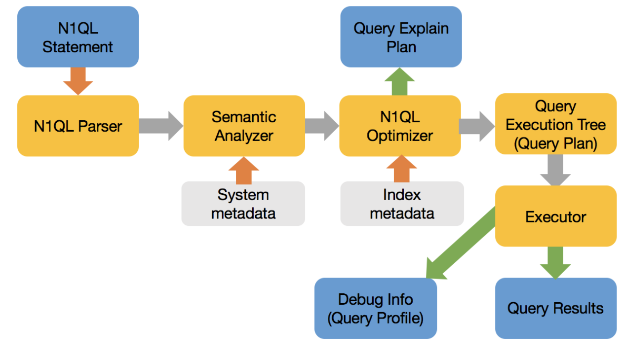
El optimizador, a grandes rasgos, hace lo siguiente:
- Reescriba la consulta a su forma equivalente óptima para facilitar la optimización y sus elecciones.
- Seleccionar la vía de acceso para cada espacio de claves (equivalente a las tablas)
- Seleccione uno o varios índices para cada espacio de claves.
- Seleccione el orden de unión para todas las uniones en la cláusula FROM. N1QL Optimizer aún no reordena las uniones.
- Seleccione el tipo de unión (por ejemplo, bucle anidado o unión hash) para cada unión
- Por último, cree el árbol de ejecución de la consulta (plan).
En este documento hemos descrito el optimizador basado en reglas de N1QL: Una inmersión profunda en la optimización de consultas N1QL de Couchbase.
Aunque en este artículo se habla principalmente de las sentencias SELECT, el CBO elige planes de consulta para las sentencias UPDATE, DELETE, MERGE e INSERT (en con SELECT). Los retos, la motivación y la solución son igualmente aplicables a todas estas sentencias DML.
N1QL dispone de los siguientes métodos de acceso:
- Exploración de valores
- Escaneo de llaves
- Exploración de índices
- Escaneado del índice de cobertura
- Exploración primaria
- Unión de bucles anidados
- Unión hash
- Escaneo indecoroso
Motivación de un optimizador basado en costes (OBC)

¿Imaginas que google maps te diera la misma ruta independientemente de la situación actual del tráfico? Un enrutamiento basado en costes tiene en cuenta el coste actual (tiempo estimado basado en el flujo de tráfico actual) y encuentra la ruta más rápida. Del mismo modo, un optimizador basado en costes tiene en cuenta la cantidad probable de procesamiento (memoria, CPU, E/S) para cada operación, estima el coste de las rutas alternativas y selecciona el plan de consulta (árbol de ejecución de consultas) con el menor coste. En el ejemplo anterior, el algoritmo de enrutamiento tiene en cuenta la distancia, el tráfico y te da las tres mejores rutas.
Para los sistemas relacionales, CBO fue inventado en 1970 en IBM, descrito en este artículo de referencia. En el actual optimizador basado en reglas de N1QL, las decisiones de planificación son independientes de la inclinación de los datos para varias rutas de acceso y de la cantidad de datos que califican para los predicados. Esto resulta en una generación inconsistente del plan de consulta y un rendimiento inconsistente porque las decisiones pueden ser menos que óptimas.
Hay muchas bases de datos JSON: MongoDB, Couchbase, Cosmos DB, CouchDB. Muchas bases de datos relacionales soportan el tipo JSON y funciones de acceso para indexar y acceder a los datos dentro de JSON. Muchas de ellas, Couchbase, CosmosDB, MongoDB tienen un lenguaje de consulta declarativo para JSON y hacen selección de rutas de acceso y generación de planes. Todos ellos implementan optimizadores basados en reglas heurísticas. Aún no hemos visto ningún documento o documentación que indique un optimizador basado en costes para ninguna base de datos JSON.
En el mundo NoSQL y Hadoop, existen algunos ejemplos de optimizadores basados en costes.
Pero, estos sólo manejan los tipos escalares básicos, al igual que el optimizador de base de datos relacional. No gestionan el cambio de tipos, el cambio de esquema, los objetos, las matrices y los elementos de matrices, todos los cuales son cruciales para el éxito del lenguaje de consulta declarativo sobre JSON.
|
1 2 3 4 5 6 7 8 9 10 11 12 13 14 15 16 17 18 19 20 |
Considere el cubo cliente: /* Crear algunos índices */ CREAR PRIMARIO índice EN cliente; CREAR ÍNDICE ix1 EN cliente(nombre, cremallera, estado); CREAR ÍNDICE ix2 EN cliente(zip, nombre, estado); CREAR ÍNDICE ix3 EN cliente(zip, estado, nombre); CREAR ÍNDICE ix4 EN cliente(nombre, estado, zip); CREAR ÍNDICE ix5 EN cliente(estado, cremallera, nombre); CREAR ÍNDICE ix6 EN cliente(estado, nombre, zip); CREAR ÍNDICE ix7 EN cliente(estado); CREAR ÍNDICE ix8 EN cliente(nombre); CREAR ÍNDICE ix9 EN cliente(zip); CREAR ÍNDICE ix10 EN cliente(estado, nombre); CREAR ÍNDICE ix11 EN cliente(estado, zip); CREAR ÍNDICE ix12 EN cliente(nombre, zip); |
Ejemplo de consulta:
SELECCIONAR * DESDE cliente WHERE nombre = "Joe" AND zip = 94587 AND status = "Premium";
La pregunta es sencilla:
- Todos los índices anteriores son vías de acceso válidas para evaluar la consulta. ¿Cuál de los varios índices debería usar N1QL para ejecutar la consulta eficientemente?
- La respuesta correcta es, depende. Depende de la cardinalidad, que a su vez depende de la distribución estadística de los datos de cada clave.
Podría haber un millón de personas con el nombre Joe, diez millones de personas en el código postal 94587 y sólo 5 personas con estatus Premium. Podría haber pocas personas con el nombre Joe o más personas con estatus Premium o menos clientes en el código postal 94587. El número de documentos que cumplen los requisitos de cada filtro y las estadísticas combinadas afectan a la decisión.
Hasta aquí, los problemas son los mismos que los de la optimización SQL. Seguir este enfoque es seguro para recopilar estadísticas, calcular selectividades y elaborar el plan de consulta.
Pero JSON es diferente:
- El tipo de datos puede cambiar entre varios documentos. Zip puede ser numérico en un documento, cadena en otro, el objeto en el tercero. ¿Cómo recopilar estadísticas, almacenarlas y utilizarlas eficazmente?
- Puede almacenar complejos, una estructura anidada utilizando matrices y objetos. ¿Qué significa recopilar estadísticas sobre estructuras anidadas, matrices, etc.?
Cicatrices: números, booleano, cadena, null, missing. En el documento siguiente, a, b, c,d, e son todos escalares.
{ "a": 482, "b": 2948.284, "c": "Hola, Mundo", "d": null, "e": missing }
Objetos:
- Búsqueda de objetos completos
- Búsqueda de elementos dentro de un objeto
- Buscar el valor exacto de un atributo dentro de los objetos
- Haga coincidir los elementos, matrices y objetos en cualquier lugar de la jerarquía.
Esta estructura sólo se conoce después de que el usuario especifique las referencias a las mismas en la consulta. Si estas expresiones están en predicados, sería bueno saber si realmente existen y luego determinar su selectividad.
He aquí algunos ejemplos.
Objetos:
- Hacer referencia a un escalar dentro de un objeto. Por ejemplo: Nombre.fname, Nombre.lname
- Hacer referencia a un escalar dentro de un array de un objeto. Por ejemplo: Facturación[*].estado
- Caso anidado de (1), (2) y (3). Utilizando UNNEST operación.
- Referirse a un objeto o a una matriz en los casos (1) a (4).
Matrices:
- Empareja el conjunto completo.
- Emparejar elementos escalares de una matriz con los tipos admitidos (número, cadena, etc.)
- Empareja objetos dentro de un array.
- Emparejar los elementos dentro de una matriz de una matriz.
- Haga coincidir los elementos, matrices y objetos en cualquier lugar de la jerarquía.
Expresiones LET:
- Necesidad de obtener selectividad en las expresiones utilizadas en la cláusula WHERE.
Operación UNNEST:
- Selectividades en los filtros en UNNESTed doc para ayudar a escoger el índice correcto (array).
JOINs: INTERIOR, EXTERIOR IZQUIERDA, EXTERIOR DERECHA
- Únete a las selectividades.
- Suele ser un gran problema también en RDBMS. Puede que no lo sea en v1.
Predicados:
- UTILIZAR TECLAS
- Comparación de valores escalares: =, >, =, <=, BETWEEN, IN
- Predicados de matriz: ANY, EVERY, ANY & EVERY, WITHIN
- Subconsultas
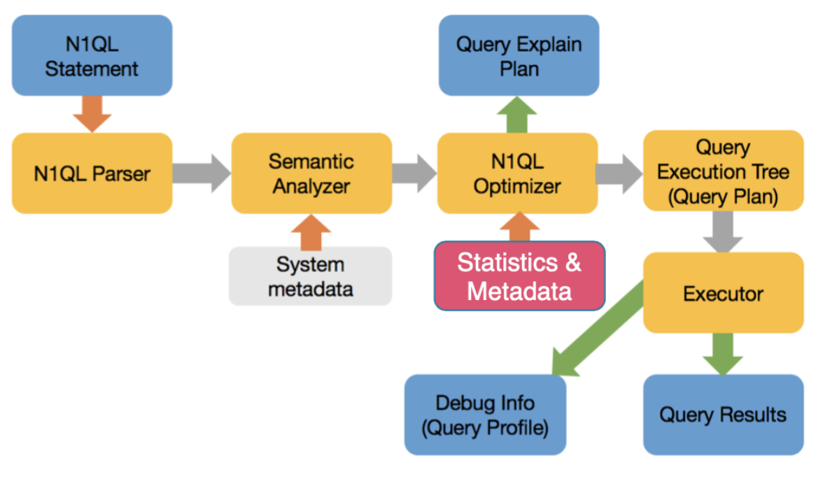
Optimizador basado en costes para N1QL
El optimizador basado en el coste estimará ahora el coste basándose en las estadísticas disponibles sobre los datos, el índice, calculará el coste de cada operación y elegirá el mejor camino.
Retos del optimizador basado en costes para JSON
- Recopilar estadísticas sobre escalares, objetos, matrices, elementos de matrices: cualquier cosa a la que se pueda aplicar un predicado (filtro).
- Crear la estructura de datos adecuada para almacenar las estadísticas de un campo cuyo tipo puede variar de un tipo a otro.
- Crear métodos para utilizar las estadísticas con el fin de calcular eficazmente estimaciones precisas sobre el complejo conjunto de estadísticas recopiladas anteriormente.
- Utilice las estadísticas adecuadas, tenga en cuenta las rutas de acceso válidas y cree un plan de consulta.
- Un campo puede ser un número entero en un documento, una cadena en el siguiente, una matriz en otro y desaparecer en otro. Los histogramas
Aproximación al optimizador basado en costes N1QL
El optimizador N1QL se encargará de determinar la estrategia de ejecución más eficiente para una consulta. Normalmente existe un gran número de estrategias de evaluación alternativas para una consulta dada. Estas alternativas pueden diferir significativamente en su requerimiento de recursos del sistema y/o tiempo de respuesta. Un optimizador de consultas basado en el coste utiliza un sofisticado motor de enumeración (es decir, un motor que enumera el espacio de búsqueda de planes de acceso y unión) para generar eficientemente una profusión de estrategias alternativas de evaluación de consultas y un modelo detallado del coste de ejecución para elegir entre esas estrategias alternativas.
El trabajo del Optimizador N1QL puede clasificarse en estas categorías:
- Recopilar estadísticas
- Recopilar estadísticas sobre campos individuales y crear un histograma único para cada campo (incluidos todos los tipos de datos que puedan aparecer en este campo).
- Recopilar estadísticas sobre cada índice disponible.
- Reescritura de consultas.
- Reescritura de consultas basada en reglas básicas.
- Estimaciones de cardinalidad
- Utilice las estadísticas de histograma e índice disponibles para estimar la selectividad.
- Utilice esta selectividad para estimar la cardinalidad
- Esto no es tan sencillo en el caso de las matrices.
- Únete al pedido.
- CONSIDER a consulta: a JOIN b JOIN c
- Es lo mismo que ( b JOIN a JOIN c), (a JOIN c JOIN b), etc.
- La elección del orden adecuado influye enormemente en la consulta.
- La implementación de Couchbase 6.5 todavía no lo hace. Este es un problema bien entendido para el que podemos tomar prestadas soluciones de SQL. JSON no introduce nuevos problemas. Los predicados de la cláusula ON pueden incluir predicados de array. Esto está en la hoja de ruta.
- CONSIDER a consulta: a JOIN b JOIN c
- Tipo de unión
- El optimizador basado en reglas utiliza bucles anidados en bloque por defecto. Es necesario utilizar directivas para forzar la unión hash. La directiva también necesita especificar el lado build/probe. Ambos son indeseables.
- CBO debe seleccionar el tipo de unión. Si se elige una unión hash, debería elegir automáticamente el lado de construcción y el lado de sondeo. Elegir el mejor espacio de claves interno/externo para el bucle anidado también está en nuestra hoja de ruta.
Recogida de estadísticas para N1QL CBO
Las estadísticas del optimizador son una parte esencial de la optimización basada en costes. El optimizador calcula los costes de varios pasos de la ejecución de la consulta, y el cálculo se basa en los conocimientos del optimizador sobre varios aspectos de las entidades físicas del servidor, lo que se conoce como estadísticas del optimizador.
Manipulación de tipos mixtos
A diferencia de las bases de datos relacionales, un campo en un documento JSON no tiene un tipo, es decir, pueden existir diferentes tipos de valores en el mismo campo. Por lo tanto, una distribución debe manejar distintos tipos de valores. Para evitar confusiones, colocamos distintos tipos de valores en distintos bins de distribución. Esto significa que podemos tener ubicaciones parciales (como la última ubicación) para cada tipo. También hay un tratamiento especial de los valores MISSING, NULL, TRUE y FALSE. Estos valores (si están presentes) siempre residen en un contenedor de desbordamiento. N1QL ha predefinido el orden de clasificación para los diferentes tipos y MISSING/NULL/TRUE/FALSE aparece al principio del flujo ordenado.
estadísticas de recogida
Para las colectas o cubos, nos reunimos:
- número de documentos de la colección
- tamaño medio del documento
Estadísticas del índice
Para un índice GSI, reunimos:
- número de elementos del índice
- número de páginas del índice
- ratio de residentes
- tamaño medio de los artículos
- tamaño medio de página
Estadísticas de distribución
Para determinados campos también recopilamos estadísticas de distribución, lo que permite una estimación más precisa de la selectividad para predicados como "c1 = 100", o "c1 >= 20", o "c1 < 150". También produce estimaciones de selectividad más precisas para predicados de unión como "t1.c1 = t2.c2", suponiendo que existan estadísticas de distribución tanto para t1.c1 como para t2.c2.
Recopilación de estadísticas del optimizador
Aunque nuestra visión es que el servidor actualice automáticamente las estadísticas necesarias del optimizador, para la implementación inicial las estadísticas del optimizador se actualizarán mediante un nuevo comando UPDATE STATISTICS.
ACTUALIZACIÓN ESTADÍSTICAS [PARA] <referencia_espacio_clave> (<expresiones_índice>) [CON <opciones>]
es un nombre de colección (puede que también admitamos bucket, aún no se ha decidido).
El comando anterior sirve para recopilar estadísticas de distribución, es una o más expresiones (separadas por comas) para las que se deben recopilar estadísticas de distribución. Soportamos las mismas expresiones que en el comando CREATE INDEX, por ejemplo, un campo, un campo anidado (dentro de objetos anidados, por ejemplo location.lat), una expresión ALL para matrices, etc.La cláusula WITH es opcional, si está presente, especifica opciones para el comando UPDATE STATISTICS. Las opciones se especifican en formato JSON de forma similar a como se especifican las opciones para otros comandos como CREATE INDEX o INFER.
Actualmente se admiten las siguientes opciones en la cláusula WITH:
- tamaño_muestrapara recopilar estadísticas de distribución, el usuario puede especificar el tamaño de la muestra que desea utilizar. Se trata de un número entero. Tenga en cuenta que también calculamos un tamaño mínimo de la muestra y tomamos el mayor entre el tamaño de la muestra especificado por el usuario y el tamaño mínimo de la muestra calculado.
- resoluciónpara recopilar estadísticas de distribución, indique cuántos bins de distribución se desean (granularidad de los bins de distribución). Se especifica como un número flotante, tomado como porcentaje. Por ejemplo, {"resolución": 1.0} significa que cada bandeja de distribución contiene aproximadamente el 1 por ciento del total de documentos, es decir, se desean ~100 bandejas de distribución. La resolución por defecto es 1,0 (100 contenedores de distribución). Se aplicará una resolución mínima de 0,02 (5000 contenedores de distribución) y una resolución máxima de 5,0 (20 contenedores de distribución).
- update_statistics_timeoutpuede especificarse un valor de tiempo de espera (en segundos). El comando ACTUALIZAR ESTADÍSTICAS finaliza con un error cuando se alcanza el tiempo de espera. Si no se especifica, se calculará un valor de tiempo de espera por defecto basado en el número de muestras utilizadas.
Manipulación de tipos mixtos
A diferencia de las bases de datos relacionales, un campo en un documento JSON no tiene un tipo, es decir, pueden existir diferentes tipos de valores en el mismo campo. Por lo tanto, una distribución debe manejar distintos tipos de valores. Para evitar confusiones, colocamos distintos tipos de valores en distintos bins de distribución. Esto significa que podemos tener ubicaciones parciales (como la última ubicación) para cada tipo. También hay un tratamiento especial de los valores MISSING, NULL, TRUE y FALSE. Estos valores (si están presentes) siempre residen en un contenedor de desbordamiento. N1QL ha predefinido el orden de clasificación para los diferentes tipos y MISSING/NULL/TRUE/FALSE aparece al principio del flujo ordenado.
Papeleras
Dado que sólo conservamos el valor máximo de cada recipiente, el límite mínimo se obtiene a partir del valor máximo del recipiente anterior. Esto también significa que la primera bandeja de distribución no tiene un valor mínimo. Para solucionarlo, colocamos un "contenedor límite" al principio, un contenedor especial de tamaño 0 cuyo único propósito es proporcionar un valor máximo, que es el límite mínimo del siguiente contenedor de distribución.
Dado que una distribución puede contener varios tipos, separamos los tipos en distintos intervalos de distribución y también colocamos un "intervalo límite" para cada tipo, de forma que conozcamos el valor mínimo de cada tipo en una distribución.
Ejemplo de tratamiento de tipos mixtos y depósitos delimitadores
ACTUALIZACIÓN ESTADÍSTICAS para CLIENTE(cantidad);
Histograma: Número total de documentos: 5000 con cantidad en números enteros simples.
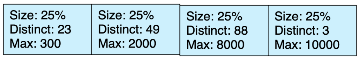
Predicados:
-
(cantidad = 100): Estimación 1%
-
(cantidad entre 200 y 100) : Presupuesto 20%
También utilizamos técnicas adicionales como mantener los valores más alto/segundo más alto, más bajo, segundo más bajo para cada bandeja, mantener una bandeja de desbordamiento para los valores que se producen más de 25% de las veces para mejorar este cálculo de selectividad.
En JSON, cantidad puede ser cualquiera de los tipos: MISSING, null, boolean, integer, string, array y un objeto. Para simplificar, mostramos el histograma de cantidad con tres tipos: enteros, cadenas y matrices. Se ha ampliado para incluir todos los tipos.
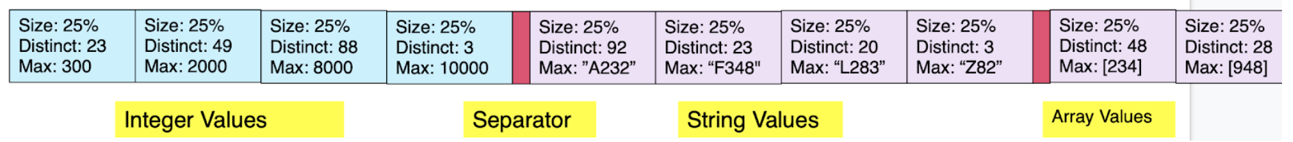
N1QL define el método mediante el cual se pueden comparar valores de distintos tipos.
- Orden de los tipos: de menor a mayor
- Falta < null < false < true < numeric < string < array < object
- Después de muestrear los documentos, primero los agrupamos por tipos, los clasificamos dentro del grupo de tipos y creamos el mini-histograma de cada tipo.
- A continuación, unimos estos mini-histogramas en un gran histograma con un límite entre cada tipo. Esto ayuda al optimizador a calcular selectividades de forma eficiente, ya sea en un solo tipo o en varios.
Ejemplos:
|
1 2 3 4 5 6 7 8 |
DONDE cantidad entre 100 y 1000; DONDE cantidad entre 100 y "4829"; DONDE cantidad entre 100 y [235]; DONDE cantidad entre 100 y {"val": "2829"}; |
Las estadísticas de distribución para tipos de datos simples son sencillas. Los valores booleanos tendrán dos intervalos de desbordamiento que almacenarán los valores TRUE y FALSE. Los valores numéricos y de cadena también son fáciles de manejar. Queda pendiente la cuestión de si queremos limitar el tamaño de un valor de cadena como límite de una bandeja, es decir, si una cadena es muy larga, ¿queremos truncar la cadena antes de almacenarla como valor máximo para una bandeja de distribución? Los valores de cadena largos en una bandeja de desbordamiento no se truncarán, ya que eso requiere una coincidencia exacta.
El diseño de cómo recoger las estadísticas de distribución no se ha finalizado. Lo que queremos hacer es probablemente recopilar estadísticas de distribución en elementos individuales del array, ya que así es como funciona el índice del array. Puede que necesitemos soportar las variaciones DISTINCT/ALL del índice del array incluyendo la misma palabra clave delante de la especificación del campo del array, que determina si eliminamos los duplicados del array antes de construir el histograma.
Estimar la selectividad de un predicado de matriz (CUALQUIER predicado) basándose en un histograma de este tipo es un poco complicado. No es fácil tener en cuenta las longitudes variables de las matrices de la colección. En la primera versión, nos limitaremos a mantener un tamaño medio de array como parte de las estadísticas de distribución. Esto supone algún tipo de uniformidad, lo que ciertamente no es lo ideal, pero es un buen comienzo.
Estimar la selectividad de TODOS los predicados es aún más complicado, puede que necesitemos utilizar algún tipo de valor por defecto para esto.
Considere este documento JSON en el espacio de claves
|
1 2 3 4 5 6 7 8 9 10 11 12 |
{ "a": 1, "b": [ 5, 10, 15,20,5,20,10], "c": [ { "x": "hola", "y": verdadero }, { "x": "gracias", "y": falso} ] } |
El campo "a" es un escalar, b es un array de escalares y c es un array de objetos. Cuando se emite una consulta, se pueden tener predicados en cualquiera de los campos o en todos ellos: a, b, c. Hasta ahora hemos hablado de los escalares cuyo tipo puede cambiar. Ahora vamos a hablar de la recopilación de estadísticas de predicados de array y del cálculo de selectividad.
|
1 2 3 4 5 6 7 8 9 10 11 12 13 14 |
Matriz predicados: DESDE k DONDE CUALQUIER e EN b SATISFACE e = 10 FIN DESDE k DONDE CUALQUIER e en b SATISFACE e > 50 FIN DESDE k DONDE CUALQUIER e EN b SATISFACE e ENTRE 30 y 100 FIN DESDE k UNNEST k.b AS e DONDE e = 10; DESDE k UNNEST k.b AS e DONDE e > 10; DESDE k DONDE CUALQUIER f EN c SATISFACE e.x = "hola" FIN DESDE k DONDE CUALQUIER f EN c SATISFACE e.y = verdadero FIN DESDE k UNNEST k.c AS f DONDE f.x = "gracias" |
Se trata de predicados sencillos sobre matrices de escalares y matrices de objetos. Se trata de una implementación generalizada en la que la consulta puede escribirse para filtrar elementos y valores en matrices de matrices, matrices de objetos de matrices, etc.
Cuando se tienen mil millones de estos documentos, se crean índices de matrices para ejecutar eficientemente el filtro. Ahora, para el optimizador, es importante estimar el número de documentos que cumplen los requisitos para un predicado determinado.
|
1 2 3 4 5 6 7 8 9 |
CREAR ÍNDICE i1 EN k(DISTINTO b); CREAR ÍNDICE I2 EN k (TODOS b); CREAR ÍNDICE i3 EN k(DISTINTO matriz f.x para f EN c) CREAR ÍNDICE i3 EN k(TODOS matriz f.x para f EN c) |
El índice i1 con la clave DISTINCT b crea un índice con sólo los elementos distintos (únicos) de b.
El índice i2 con la clave ALL b crea un índice con todos los elementos de b.
Esto existe para gestionar el tamaño del índice, posibilidad de obtener grandes resultados intermedios del índice. En ambos casos, habrá MÚLTIPLES entradas en el índice para CADA elemento de un array. Esto es DISTINTO a un escalar que tiene SOLO una entrada en el índice POR documento JSON.
Para obtener más información sobre la indexación de matrices, consulte documentación sobre indexación de matrices en Couchbase.
¿Cómo se recopilan estadísticas sobre esta matriz o matriz de objetos? La clave es recopilar estadísticas EXACTAMENTE en la misma expresión que la expresión en la que estás creando el índice.
En este caso, recopilamos estadísticas sobre lo siguiente:
|
1 2 3 4 5 6 7 8 |
ACTUALIZACIÓN ESTADÍSTICAS PARA k(DISTINTO b) ACTUALIZACIÓN ESTADÍSTICAS PARA k(TODOS b) ACTUALIZACIÓN ESTADÍSTICAS PARA k(DISTINTO matriz f.x para f EN c) ACTUALIZACIÓN ESTADÍSTICAS PARA k(TODOS matriz f.x para f EN c) |
Ahora bien, dentro del histograma puede haber cero, uno o varios valores procedentes del mismo documento. Por tanto, calcular la selectividad (porcentaje estimado de documentos que cumplen los requisitos del filtro) no es tan fácil.
He aquí la novedosa solución para resolver el problema con las matrices:
Para las estadísticas normales: hay una entrada de índice por documento.
La cardinalidad se convierte en un simple: selectividad x cardinalidad de la tabla;
Para las estadísticas de matrices: Hay N entradas de índice por documento;
N-> Número de valores distintos en el array.
N = 0 a n, n <= ARRAY_LENGTH(a)
Esta estadística adicional debe recogerse y almacenarse en el histograma.
Ahora, cuando se elige un índice para la evaluación de un predicado concreto, la exploración del índice devolverá todas las claves cualificadas del documento, que contienen duplicados. El motor de consulta realizará entonces una operación distinta para obtener las claves únicas y obtener los resultados correctos (no duplicados). El optimizador basado en costes tendrá que tener esto en cuenta al calcular el número de documentos (no el número de entradas del índice) que calificarán el predicado. Así pues, dividimos la estimación por la estimación de la longitud media del tamaño del array.
Esta cardinalidad se puede utilizar para calcular el coste y comparar el coste de utilizar la ruta matriz-índice frente a otra ruta de acceso legal para encontrar la mejor ruta de acceso.
Valores objeto, JSON y binarios
No está clara la utilidad de un histograma sobre un valor objeto/JSON o un valor binario. Debería ser raro ver comparaciones con tales valores en la consulta. Podemos tratarlos exactamente igual que otros tipos simples, es decir, poner el número de valores, el número de valores distintos y un límite máximo en cada recipiente de distribución; o podemos simplificar y simplemente poner el recuento en el recipiente de distribución sin el número de valores distintos ni el valor máximo. El problema con el valor máximo es similar al de las cadenas largas, donde el valor puede ser grande, y almacenar valores tan grandes puede no ser beneficioso en el histograma. Esto sigue siendo una cuestión abierta por ahora.
Estadísticas de campos en objetos anidados
Considere este documento JSON en el espacio de claves:
|
1 2 3 4 5 6 7 8 9 10 11 |
{ "a": 1, "b": {"p": "NY", "q": "212-820-4922", "r": 2848.23}, "c": { "d": 23, "e": { "x": "hola", "y": verdadero , "z": 48} } } |
A continuación se muestra la expresión punteada para acceder a objetos anidados.
FROM k WHERE b.p = "NY" AND c.e.x = "hola" AND c.e.z = 48;
Dado que cada camino es único, recoger y utilizar el histograma es igual que escalar.
ACTUALIZAR ESTADÍSTICAS PARA k(b.p, c.e.x, c.e.z)
Resumen
Hemos descrito cómo hemos implementado un optimizador basado en costes para N1QL (SQL para JSON) y gestionado los siguientes retos.
- N1QL CBO puede manejar esquemas JSON flexibles.
- N1QL CBO puede manejar escalares, objetos y matrices.
- N1QL CBO puede manejar la recolección de estadísticas y calcular estimaciones en cualquier campo de cualquier tipo dentro de JSON.
- Todo ello mejorará los planes de consulta y, por tanto, el rendimiento del sistema. También reducirá el coste total de propiedad al reducir la sobrecarga de depuración del rendimiento del administrador de bases de datos.
- Descargar Couchbase 6.5 y pruébelo usted mismo.
Recursos Optimizador basado en reglas N1QL
El primer artículo describe el optimizador de Couchbase a partir de la versión 5.0. Añadimos uniones ANSI en Couchbase 5.5. El segundo artículo incluye su descripción y algunas de las optimizaciones realizadas para ello.
- Una inmersión profunda en la optimización de consultas N1QL de Couchbase https://dzone.com/articles/a-deep-dive-into-couchbase-n1ql-query-optimization
- Soporte ANSI JOIN en N1QL https://dzone.com/articles/ansi-join-support-in-n1ql
- Crear el índice adecuado, Obtener el rendimiento adecuado para el optimizador basado en reglas.
- Algoritmo de selección de índices
Referencias
- Selección de rutas de acceso en un sistema de gestión de bases de datos relacionales. https://people.eecs.berkeley.edu/~brewer/cs262/3-selinger79.pdf
- Optimización basada en costes en DB2 XML. http://www2.hawaii.edu/~lipyeow/pub/ibmsys06-xmlopt.pdf
- Selección de rutas de acceso en un sistema de gestión de bases de datos relacionales. https://people.eecs.berkeley.edu/~brewer/cs262/3-selinger79.pdf