Búsqueda ANN filtrada con índices vectoriales compuestos (Parte 2)

Esta es la segunda entrada de una serie de varias partes dedicada a explorar la indexación vectorial compuesta en Couchbase. Consulte la primera entrada. aquí. 

La serie tratará los siguientes temas:

1. Por qué son importantes los índices vectoriales compuestos, incluyendo conceptos, terminología y motivación de los desarrolladores. Se utilizará un sistema inteligente de recomendación de productos alimenticios como ejemplo práctico.
2. Cómo se implementan los índices vectoriales compuestos dentro del servicio de indexación de Couchbase.
3. Cómo funciona ORDER BY pushdown para consultas vectoriales compuestas.
4. Comportamiento real y resultados de pruebas comparativas.

Implementación de índices vectoriales compuestos

GSI utiliza el índice FAISS en segundo plano. Se creará una cadena de índice como la que se muestra a continuación a partir del campo de descripción proporcionado en el DDL.

Ejemplo: Con una cadena descriptiva como “IVF10000,PQ32x8”, se construirá una cadena de fábrica de índices FAISS como “IVF10000_HNSW,PQ32x8”.

Sin embargo, esta cadena de fábrica solo se utiliza como bloque de construcción durante el entrenamiento y la configuración del índice. GSI no se basa en FAISS como un índice monolítico en memoria para todo el conjunto de datos. En su lugar, FAISS se aplica de forma selectiva a los datos muestreados para aprender los centroides y los libros de códigos de cuantificación, mientras que Couchbase se encarga de gestionar el diseño completo del índice, el almacenamiento, el manejo de mutaciones y la ejecución de consultas. Esto permite a Couchbase escalar la búsqueda vectorial de manera eficiente, integrar el filtrado escalar y la semántica de las consultas, y admitir actualizaciones continuas. - capacidades que van mucho más allá de invocar un índice FAISS independiente.

Incrustaciones

La capa de incrustación toma los campos de texto relevantes, los envía a través de un modelo transformador y produce vectores semánticos que representan cada producto. Estos vectores alimentan la búsqueda ANN. La aplicación debe almacenar estas incrustaciones junto con los datos del producto para que el índice vectorial pueda utilizarlas y garantizar que las incrustaciones almacenadas coincidan con la definición del índice vectorial (por ejemplo, dimensión fija y tipo numérico) esperada por Couchbase.

Creación y construcción de índices

Crear y desarrollar el flujo

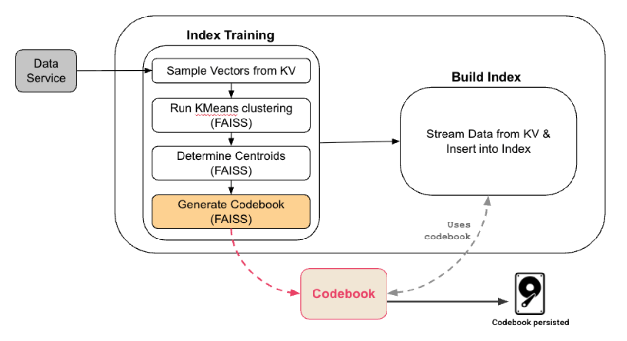
• Si el usuario tiene un número suficiente de vectores almacenados, GSI toma muestras aleatorias de los datos para crear un conjunto de datos representativo.
• Este conjunto de datos representativo se utiliza para entrenar el índice FAISS. Después del entrenamiento, GSI conserva el libro de códigos, que incluye una lista invertida IVF y libros de códigos PQ:
  • La IVF divide el espacio vectorial en nlist particiones y cada partición está representada por un centroide.
  • Se utiliza cuantificación PQ o SQ por partición para comprimir los vectores.
  • Se crea el gráfico HNSW de los centroides; resulta útil cuando el número de centroides es muy grande.
• Los datos se transmiten desde el servicio de datos utilizando el protocolo DCP y para cada documento recibido.
  • El documento se asigna a la partición cuyo centroide está más cerca del vector, es decir, el centroide es C1.
• Durante la indexación, el vector de cada documento se asigna a su centroide más cercano, se almacena en un formato compacto codificado optimizado para el cálculo rápido de distancias y se rastrea de manera eficiente, de modo que las actualizaciones futuras solo vuelvan a procesar el vector si realmente cambia.

Nota

Si la distribución vectorial subyacente cambia significativamente, el índice debe reconstruirse para volver a entrenarlo. Esto puede suceder debido a:

• Un cambio en el modelo de incrustación (por ejemplo, cambiar de modelo o de dimensiones).
• Cambios importantes en la distribución de datos (nuevas categorías de productos, cambios de idioma o desviación de dominios).
• Reincorporar documentos existentes con incorporaciones actualizadas.

¿Cuántos documentos se necesitan para entrenar un índice vectorial?

Al crear un índice vectorial, Couchbase toma automáticamente muestras de los datos vectoriales para entrenar el índice y lograr una búsqueda ANN eficiente y precisa.

En general, la colección debe contener al menos tantos documentos como el número de centroides (nlist) configurados para el índice, ya que cada centroide requiere datos de entrenamiento.

Cuando se utiliza la cuantificación de productos (PQ), este mínimo se convierte en max(nlist, 2^nbits) para garantizar datos suficientes para el entrenamiento del cuantificador, donde nbits es N de PQ{M}x{N}.

Couchbase gestiona la capacitación de la siguiente manera:

• Conjuntos de datos pequeños (hasta ~10,000 documentos):
  • Todos los vectores se utilizan para el entrenamiento, no se requiere muestreo.
• Conjuntos de datos más grandes:
  • De forma predeterminada, Couchbase selecciona un conjunto de entrenamiento tomando el mayor de los siguientes, mientras que limita el tamaño final de la muestra a 1 millón de vectores:
    • 10% del conjunto de datos, y
    • 10 veces el número de centroides (nlist)
  • Este enfoque equilibra la calidad de la capacitación con el tiempo de creación del índice.

Buenas prácticas: Para obtener un entrenamiento estable y de alta calidad, intente alcanzar al menos 10 vectores por centroide, lo que permite que el índice aprenda la distribución vectorial subyacente de manera eficaz.

Control avanzado: Si es necesario, puede controlar explícitamente el número de vectores de entrenamiento especificando el parámetro train_list al crear el índice.

Couchbase gestiona automáticamente el proceso de muestreo y entrenamiento. Como usuario, el requisito clave es asegurarse de que exista un número suficiente de documentos incrustados antes de crear el índice.

Escaneo de índice

Flujo de escaneo

Cuando llega una consulta que contiene una búsqueda vectorial, Couchbase sigue una secuencia bien definida para enrutarla a través de los componentes adecuados y preparar el escaneo.

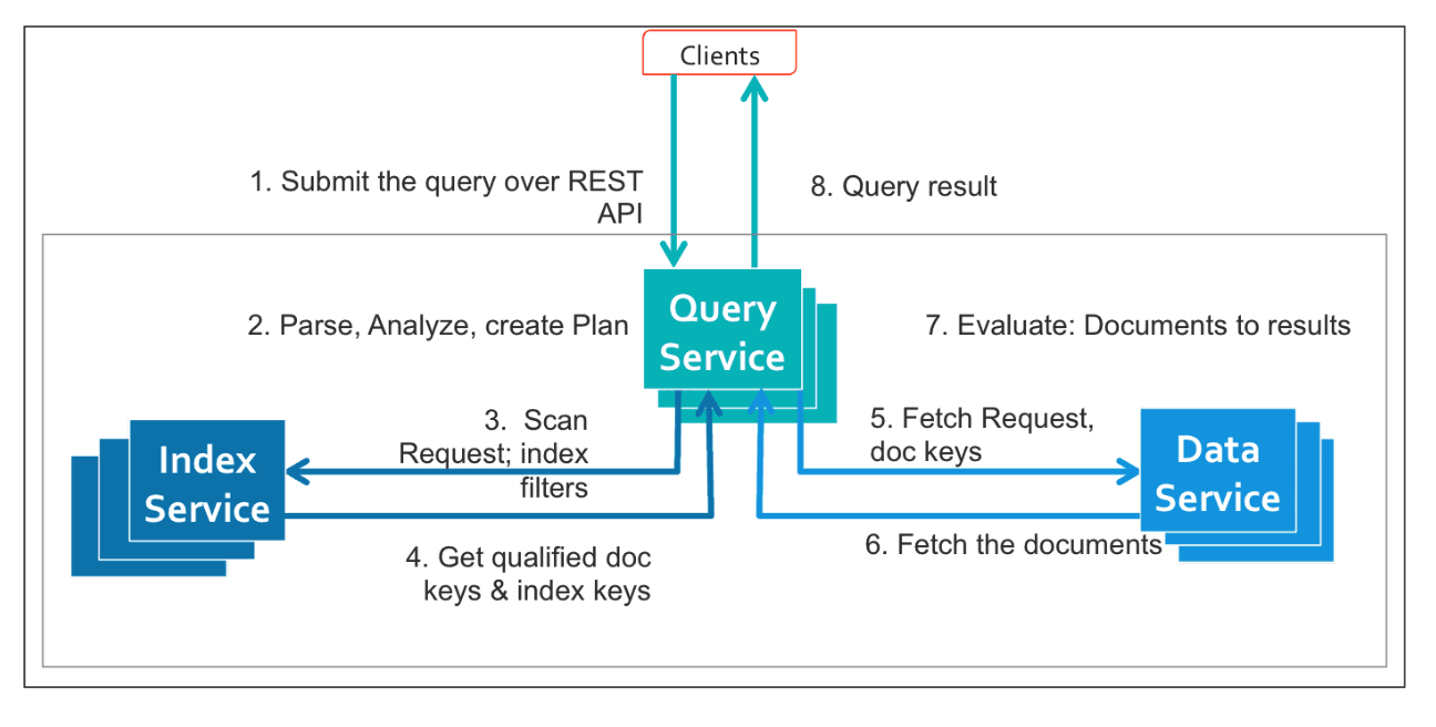
Si se han creado índices vectoriales sargables y están activos, el servicio de consulta puede utilizarlos para atender las consultas ANN filtradas más rápidamente.

El coordinador de escaneo en el proceso del indexador recibe las entradas que se mencionan a continuación junto con el nombre del índice y los parámetros de consistencia:

• Filtros escalares en campos indexados
  • Predicados de igualdad o rango como azúcares_100g < 20
• El vector de consulta
  • Incorporación de la intención de búsqueda del usuario
• El tamaño del resultado k
  • Cuántos artículos similares quiere recuperar el usuario. 
  • Esto se indica en el LÍMITE.
• El número de centroides más cercanos n
  • ¿Qué parte del espacio vectorial queremos buscar?
  • El valor n de nprobes es un parámetro para DISTANCIA_VECTOR_APROX

Después de obtener la información anterior, se crea una solicitud de escaneo, que sigue los siguientes pasos:

1. La instantánea del índice se obtiene en función de los parámetros de consistencia proporcionados.
   • Si el usuario necesita consistencia en la sesión, el indexador obtiene la última marca de tiempo del servicio de datos y espera a que el indexador se ponga al día y genere instantáneas consistentes que puedan servir para la consulta.
   • Si el usuario está de acuerdo con cualquier consistencia, el indexador utiliza la instantánea que ha almacenado en caché sin esperar.
2. El indexador espera a los lectores de almacenamiento necesarios para atender la consulta. 
   • Dado que los recursos del indexador son limitados, se configura con el número máximo de lectores que se pueden ejecutar; por lo tanto, si un sistema está ocupado, los escaneos deben esperar a que los lectores estén libres.
3. El indexador recupera los libros de códigos para las particiones que se están escaneando para la consulta dada.
   • Tenga en cuenta que el libro de códigos (lista invertida IVF y libros de códigos PQ) no cambia después de la fase de entrenamiento inicial, por lo que no hay instantáneas para el libro de códigos.
4. Utilizando los libros de códigos obtenidos anteriormente, el más cercano nprobe Se obtienen los centroides del vector de consulta en cada partición necesaria para un vector de consulta dado.
5. Para una partición de índice determinada, los filtros escalares y los centroides más cercanos se combinan para formar rangos de exploración sin superposición para leer datos del índice.
6. Ahora, el indexador configura un canal de exploración dedicado. Piensa en este canal como una pequeña cadena de montaje de corta duración creada específicamente para esa consulta. Las etapas del canal (lectura, acumulación y escritura) se ejecutan en paralelo para acelerar el proceso de consulta.

Escanear canalización

El proceso de escaneo en sí mismo tiene tres etapas: lectura, agregación y escritura. Como cualquier proceso, cada etapa se ejecuta en paralelo y transmite su resultado a la siguiente.

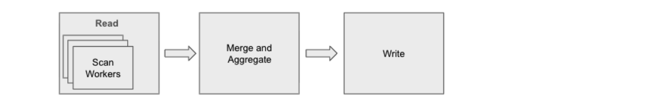
1. Etapa de lectura => Escaneo paralelo + Filtrado escalar
   • La etapa de lectura se distribuye entre varios trabajadores de escaneo.
   • Cada trabajador:
     • Escanea y lee el rango de índices que se le ha asignado.
     • Aplica filtros escalares desde el principio para eliminar elementos irrelevantes.
     • Solo envía los documentos que cumplen los requisitos a la siguiente etapa.
   • Esta poda temprana es crucial, ya que evita cálculos innecesarios de la distancia vectorial más adelante.
2. Etapa agregada => Ordenación + Cálculo de distancia vectorial
   • La etapa agregada recopila los resultados de todos los trabajadores y realiza el “trabajo pesado”.”
   • Combina y ordena los elementos si es necesario.
   • Sustituye las distancias aproximadas basadas en el centroide por distancias reales calculadas.
   • Mantiene un montón top-k para rastrear a los mejores candidatos hasta el momento.
   • En esta etapa es donde la lógica ANN se une al filtrado escalar.
3. Etapa de escritura => Transmisión de resultados al cliente GSI en el servicio de consulta
   • Por último, la etapa de escritura transmite los resultados agregados al Servicio de Consultas.
   • Si el índice se distribuye entre varios nodos indexadores, se fusionan los resultados de cada nodo.
   • A partir de ahí, el procesador de consultas puede realizar operaciones adicionales, tales como:
     • Filtrado de grano grueso
     • Se une a
     • Proyecciones o clasificación final

El usuario recibe finalmente una lista clara y ordenada de los vecinos más cercanos que cumplen todas las condiciones escalares.

Comportamiento avanzado de consultas en exploraciones de índices vectoriales compuestos

Una vez que comprenda cómo funciona un canal de exploración vectorial, hay varios conceptos más profundos que influyen en la eficiencia con la que se ejecutan sus consultas. Estos comportamientos están relacionados con cómo se define el índice y cómo interactúan los predicados escalares con las particiones vectoriales.

Paralelismo de escaneo

Cada consulta tiene un límite natural en cuanto al paralelismo que puede aprovechar. Este paralelismo inherente proviene de la cantidad de rangos de índices no superpuestos que se pueden generar a partir de los predicados escalares y las nprobes. Cuantos más rangos disjuntos haya, más oportunidades habrá de realizar escaneos en paralelo.

Pero las restricciones escalares no son el único factor. El número real de trabajadores que utiliza el sistema es el mínimo de:

• Cuánto paralelismo inherente puede exponer la consulta
• Cuántos centroides necesita buscar la consulta.
• Cuántos centroides contiene el índice.
• El número máximo de trabajadores configurados por escaneo por partición.

Esto evita que el sistema sobrecargue la CPU o cree subprocesos innecesarios cuando no hay trabajo paralelo adicional que realizar.

Predicados clave principales - Donde comienza el paralelismo

Los predicados de las claves del índice principal (los primeros campos que aparecen en la definición del índice compuesto) determinan el grado de paralelismo que puede aprovechar la consulta.

Si una clave escalar principal tiene varios predicados de igualdad, cada uno se convierte en un rango de exploración independiente, lo que permite al sistema distribuirlos y ejecutarlos en paralelo.

Si la clave principal utiliza un predicado de rango, toda la consulta se reduce a un gran rango de exploración, lo que reduce el paralelismo.

En resumen:

• Igualdad en las claves principales → paralelismo máximo
• Rango en las claves principales → un gran escaneo secuencial

La elección de las claves principales adecuadas en la definición del índice tiene un impacto directo en la latencia.

Los predicados vectoriales se comportan efectivamente como filtros de igualdad en los ID de centroides, seleccionando un conjunto fijo de clústeres para escanear.

Selectividad escalar - Cuánto trabajo no tienes que hacer

La selectividad escalar mide cuántos puntos de datos pueden eliminarse mediante un filtro escalar.

Un filtro altamente selectivo elimina una gran parte del conjunto de datos antes incluso de que comiencen los cálculos de distancia vectorial.

Por ejemplo:

• azúcares_100g < 20 puede eliminar 70% de artículos
• proteínas_100 g > 10 puede eliminar 90% de artículos

Cuanto más selectivo sea el escalar, menos vectores deberá comparar el índice.

El rendimiento del escaneo del índice vectorial compuesto aumenta proporcionalmente con la selectividad escalar, ya que el proceso dedica menos tiempo a leer documentos y calcular distancias.

Paginación - Resultados vectoriales ordenados

Los escaneos de índice vectorial compuesto producen un orden global para el conjunto de resultados.

Esto ocurre porque el índice sustituye los ID de centroides por distancias vectoriales reales, lo que proporciona a cada candidato una métrica de distancia precisa.

Puede utilizar LIMIT y OFFSET para paginar los resultados siempre que existan suficientes elementos que cumplan los requisitos dentro de los n centroides seleccionados.

Esto hace que los índices vectoriales compuestos sean adecuados para interfaces de usuario que requieren desplazamiento infinito o navegación por productos página por página.

Flexibilidad en la definición del índice - Adapte el índice a la carga de trabajo

El índice vectorial compuesto DDL le ofrece un control total sobre el orden de las claves de índice.

Esta orden afecta directamente a cómo se realiza el filtrado, lo que a su vez repercute en el rendimiento de la consulta.

Esta flexibilidad permite múltiples estrategias de poda:

• Poda centrada en vectores
  • Inicie el índice con la clave vectorial, seguida de los escalares:
    • CREAR ÍNDICE idx EN alimentos(vector_texto, azúcares_100g, proteínas_100g)
  • Ideal para cargas de trabajo impulsadas principalmente por la similitud vectorial.
• Poda centrada en escalares
  • Coloque primero los campos escalares altamente selectivos y, a continuación, la clave vectorial:
    • CREAR ÍNDICE idx EN alimentos(azúcares_100g, proteínas_100g, vector_de_texto)
  • Este es el patrón más común y más eficiente, ya que los escalares selectivos podan agresivamente antes de que comience la evaluación vectorial.
• Poda solo vectorial
  • Crear un índice solo en la clave vectorial:
    • CREAR ÍNDICE idx EN food(vector_de_texto)
  • Esto resulta útil cuando los campos escalares tienen poca selectividad y no ayudan a reducir el espacio de búsqueda.
• Poda solo escalar
  • Cree un índice tradicional no vectorial para las consultas que no utilicen similitud vectorial.

Compatibilidad con consultas solo escalares y escaneos de cobertura

Cuando los predicados escalares de una consulta son sargables con respecto a las claves escalares de un índice vectorial compuesto, el índice se puede utilizar para atender consultas puramente escalares. - incluso cuando no existe ninguna condición de similitud vectorial. En tales casos, el índice vectorial compuesto se comporta como un índice secundario tradicional y puede actuar como un índice de cobertura, lo que permite satisfacer la consulta íntegramente desde el índice sin necesidad de recuperar documentos del servicio de datos.

La consulta solo escalar:

Es apto para: 

Y no para:

Esto se debe a que: 

• La clave principal es un vector.
• GSI no puede buscarlo ni escanearlo.
• El índice no se puede utilizar de manera eficiente para predicados escalares.

Hasta ahora, hemos visto cómo los índices vectoriales compuestos combinan de manera eficiente la poda escalar con la similitud vectorial. Sin embargo, la similitud por sí sola rara vez es suficiente en aplicaciones reales. ¿Qué sucede cuando se desean resultados que sean semánticamente cercanos a una consulta y ordenados según señales específicas de la aplicación, como la nutrición, el precio o la frescura, sin tener que recuperar grandes conjuntos de resultados en la capa de consulta?

En la siguiente parte de esta serie, profundizaremos en Búsqueda ANN filtrada con índices vectoriales compuestos y muestra cómo Couchbase introduce la compleja semántica de ORDER BY y LIMIT directamente en el indexador, lo que permite evaluar la similitud basada en la distancia y el orden escalar juntos en una única ruta de ejecución eficiente.