ELT processing with Couchbase and N1QL

Moving data between data sources. This is one of the key activities in data integration projects. Traditionally, techniques around data movement has been part of Data Warehouse, BI and analytics. More recently Big Data, Data Lakes, Hadoop, are frequent players in this area.

In this entry, we will discuss how Couchbase N1QL language can be used to make massive manipulation on the data in this kind of scenarios.

First, let us remember the two classical approaches when doing data movement:

ETL (Extract-Transform-Load). With this model the data is extracted (from the original data source), transformed (data is reformatted to fit in the target system) and loaded (in the target data store).

ELT (Extract- Load-Transform). With this model the data is extracted (from the original data source), loaded in the same format in the target system. Then we do a transformation in the target system to obtain the desired data format.

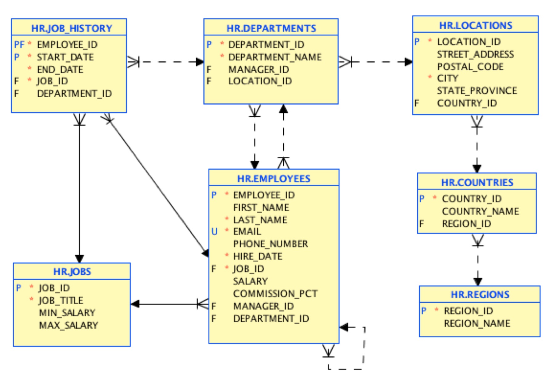
We will focus in a ELT exercise in this example. Let us do a simple export from a relational database, and load the data into Couchbase. We will use Oracle Database as input data source, with the classical HR schema example built in, which models a Human Resources department.

This is the source data model:

In the first step, we will load the data with the same structure. There is a free tool you can use to perform this initial migration here. At the end, we will have JSON documents mapping this table model:

For example, a location document will look like this:

This was an easy first step. However, this mapping table-to-document is often a bad design in the NoSQL world. In NoSQL is frequent to de-normalize your data in favour of a more direct access path, embedding referenced data. The goal is to minimize database interactions and joins, looking for the best performance.

Let us assume that our use case is driven by a frequent access to the whole job history for employees. We decide to change our design to this one:

For locations, we are joining in a single location document the referenced data for country and region.

For the employee document, we will embed the department data, and will include an array with the whole job history or each employee. This array support in JSON is a good improvement over foreign key references and joins in the relational world.

For the job document, we will maintain the original table structure.

So we have extracted and loaded the data, now we will transform into this model to finish our ELT example. How can we do this job? It is time for N1QL

N1QL is the SQL-like language included with Couchbase for data access and data manipulation. In this example, we will use two buckets: HR, which maps to the original Oracle HR schema, and HR_DNORM which will hold our target document model.

We have already loaded our HR schema. Next step is to create a bucket named HR_DNORM. Then we will create a primary index in this new bucket:

 

Now it is time for creating the location documents. This documents are composed of original locations, country and region documents:

Few things to notice:

• We are using here the projection of a SELECT statement to make the insert. In this example, the original data comes from a different bucket.
• JOINs are used in the original bucket to reference countries and regions
• IFNULL function used to set explicitly null value for the field state_province
• TO_STRING function applied on a number field to reference a key

 

Our original sample becomes this:

Note we got rid of our references location_id and country_id.

Now it is time for our employee documents. We will do it in several steps. First one is to create the employees from the original HR bucket, including department and actual job information:

Second, we will use a temporary construction to build the job history array:

Now is easy to update our employees documents adding a job_history array:

This is how our employee document looks like:

Note the job_history array of previous positions.

We can delete now the temporary job_history documents:

As last step we insert the original jobs documents:

We are done. This is a simple example, but shows can powerful can be N1QL data manipulation. Happy data migration!