Authors & Engineering Team: Bingjie Miao, Keshav Murthy, Marco Greco, Prathibha Bisarahalli. Couchbase, Inc.
A rule-based optimizer knows rules for everything and cost for nothing – Oscar Wilde
Abstract
Couchbase is a distributed JSON database. It provides distributed data processing, high performance indexing and declarative query language N1QL along with search index, eventing and analytics. N1QL (Non First Normal Query Language) is SQL for JSON. N1QL is to JSON what SQL is to relations. Developers say what needs to be done and the N1QL engine will figure out the “how”. Current N1QL optimizer is a rule based optimizer. Cost Based Optimizer(CBO) for SQL was invented at IBM some 40 years ago and has been critical to the success of RDBMS and the developer/DBA productivity. NoSQL databases were invented some 10 years ago. Shortly after their invention, NoSQL databases started adding SQL-like query language with limited access paths and optimizer capabilities. Most use rule based optimizer or simply support cost based optimization on simple scalar values (strings, numbers, boolean,etc) only.
To create a CBO on JSON model, you first need to collect and organize the statistics. How do you collect, store and use statistics on JSON’s flexible schema? How do you collect statistics on objects, arrays, elements within objects? How do you use them efficiently within your optimizer?
Lukas Eder once told me, “Cost-based optimizer makes SQL fully declarative.” He has a point. Couchbase 6.5 (now GA) has Cost Based Optimizer for N1QL. This article presents the introduction of N1QL Cost Based Optimizer (CBO) in Couchbase 6.5. CBO is a patent-pending developer-preview feature. In this article, we describe on how you can use CBO as well as its implementation details.
A PDF version of this article can be downloaded here.
Table of Contents
- Abstract
- Introduction to N1QL
- Using Cost-Based Optimizer for N1QL
- N1QL Optimizer
- Cost-Based Optimizer for N1QL
- Statistics Collection for N1QL CBO
- Summary
- Resources N1QL rule-based Optimizer
- References
Introduction to N1QL
As JSON has been increasingly accepted by the information technology industry as the lingua franca for information change, there has been an exponential rise in the need for repositories that natively store, update and query JSON documents. SQL has added features manipulating JSON in SQL:2016. SQL:2016 adds new scalar and table functions to manipulate JSON. An alternative approach is to treat JSON as the data model and to design the language to operate on JSON natively. N1QL and SQL++ use the latter approach and provide natural access to scalars, objects, arrays, arrays of objects, arrays within objects and so on.
|
1 2 3 4 5 6 7 8 9 10 11 12 13 14 15 16 |
SQL:2016: From: Microsoft SQL Server. SELECT Name,Surname, JSON_VALUE(jsonCol,'$.info.address.PostCode') AS PostCode, JSON_VALUE(jsonCol,'$.info.address."Address Line 1"')+' ' +JSON_VALUE(jsonCol,'$.info.address."Address Line 2"') AS Address, JSON_QUERY(jsonCol,'$.info.skills') AS Skills FROM People WHERE ISJSON(jsonCol) > 0 AND JSON_VALUE(jsonCol,'$.info.address.Town')='Belgrade' AND Status='Active' ORDER BY JSON_VALUE(jsonCol,'$.info.address.PostCode') |
|
1 2 3 4 5 6 7 8 9 10 |
N1QL: Same query written in N1QL on the JSON model SELECT Name,Surname, jsonCol.info.address.PostCode AS PostCode, (jsonCol.info.address.`Address Line 1` + ' ' + jsonCol.`info.address.`Address Line 2`) AS Address, jsonCol.info.skills' AS Skills FROM People WHERE jsonCol.info.address.Town = 'Belgrade' AND Status='Active' ORDER BY jsonCol.info.address.PostCode |
Learn N1QL at https://query-tutorial.couchbase.com/
Couchbase Server:
Couchbase has engines supporting N1QL:
- N1QL for interactive applications in the Query service.
- N1QL for Analytics in the Analytics service.
In this article, we focus on N1QL for Query (interactive applications) implemented in the query service. All of the data manipulated by N1QL is saved in JSON within Couchbase data store managed by the data service.
To support query processing on JSON, N1QL extends the SQL language in many ways:
-
- Support for flexible schema on semi-structured self-describing JSON.
- access and manipulate elements in JSON: scalar values, objects, arrays, objects of scalar values, arrays of scalar values, arrays of objects, arrays of arrays, etc.
- Introduce a new boolean value, MISSING to represent a missing key-value pair in a document, this is distinct from a known null value. This extends the three-valued logic to four-valued logic.
- New operations for NEST and UNNEST operations to create arrays and to flatten arrays, respectively.
- Extend the JOIN operations to work with JSON scalars, objects and arrays.
- To speedup the processing of these JSON documents the global secondary indexes can be created on one or more scalar values, scalar values of arrays, nested objects, nested arrays, objects, array objects, array elements.
- Add integrated search capability using inverted search index.
Using CBO for N1QL
We’ve introduced (CBO) in Couchbase 6.5 (now GA). Let’s look at how to use the feature before delving into the details.
- CREATE a new bucket and load the data from the sample bucket travel-sample.
|
1 2 3 4 5 6 7 8 9 |
INSERT INTO hotel(KEY id, VALUE h) SELECT META().id id, h FROM `travel-sample` h WHERE type = "hotel" |
- Sample hotel document
Here’s an example hotel document. These values are scalars, objects, and arrays. A query on this will access and process on all of these fields.
|
1 2 3 4 5 6 7 8 9 10 11 12 13 14 15 16 17 18 19 20 21 22 23 24 25 26 27 28 29 30 31 32 33 34 35 36 37 38 39 40 41 42 43 44 45 46 47 48 49 50 51 52 53 54 55 56 57 58 59 60 61 62 63 64 65 66 67 68 69 70 71 72 73 74 75 76 77 |
{ "hotel": { "address": "Capstone Road, ME7 3JE", "alias": null, "checkin": null, "checkout": null, "city": "Medway", "country": "United Kingdom", "description": "40 bed summer hostel about 3 miles from Gillingham, housed in a districtive converted Oast House in a semi-rural setting.", "directions": null, "email": null, "fax": null, "free_breakfast": true, "free_internet": false, "free_parking": true, "geo": { "accuracy": "RANGE_INTERPOLATED", "lat": 51.35785, "lon": 0.55818 }, "id": 10025, "name": "Medway Youth Hostel", "pets_ok": true, "phone": "+44 870 770 5964", "price": null, "public_likes": [ "Julius Tromp I", "Corrine Hilll", "Jaeden McKenzie", "Vallie Ryan", "Brian Kilback", "Lilian McLaughlin", "Ms. Moses Feeney", "Elnora Trantow" ], "reviews": [ { "author": "Ozella Sipes", "content": "This was our 2nd trip here and we enjoyed it as much or more than last year. Excellent location across from the French Market and just across the street from the streetcar stop. Very convenient to several small but good restaurants. Very clean and well maintained. Housekeeping and other staff are all friendly and helpful. We really enjoyed sitting on the 2nd floor terrace over the entrance and \"people-watching\" on Esplanade Ave., also talking with our fellow guests. Some furniture could use a little updating or replacement, but nothing major.", "date": "2013-06-22 18:33:50 +0300", "ratings": { "Cleanliness": 5, "Location": 4, "Overall": 4, "Rooms": 3, "Service": 5, "Value": 4 } }, { "author": "Barton Marks", "content": "We found the hotel de la Monnaie through Interval and we thought we'd give it a try while we attended a conference in New Orleans. This place was a perfect location and it definitely beat staying downtown at the Hilton with the rest of the attendees. We were right on the edge of the French Quarter withing walking distance of the whole area. The location on Esplanade is more of a residential area so you are near the fun but far enough away to enjoy some quiet downtime. We loved the trolly car right across the street and we took that down to the conference center for the conference days we attended. We also took it up Canal Street and nearly delivered to the WWII museum. From there we were able to catch a ride to the Garden District - a must see if you love old architecture - beautiful old homes(mansions). We at lunch ate Joey K's there and it was excellent. We ate so many places in the French Quarter I can't remember all the names. My husband loved all the NOL foods - gumbo, jambalya and more. I'm glad we found the Louisiana Pizza Kitchen right on the other side of the U.S. Mint (across the street from Monnaie). Small little spot but excellent pizza! The day we arrived was a huge jazz festival going on across the street. However, once in our rooms, you couldn't hear any outside noise. Just the train at night blowin it's whistle! We enjoyed being so close to the French Market and within walking distance of all the sites to see. And you can't pass up the Cafe du Monde down the street - a busy happenning place with the best French dougnuts!!!Delicious! We will defintely come back and would stay here again. We were not hounded to purchase anything. My husband only received one phone call regarding timeshare and the woman was very pleasant. The staff was laid back and friendly. My only complaint was the very firm bed. Other than that, we really enjoyed our stay. Thanks Hotel de la Monnaie!", "date": "2015-03-02 19:56:13 +0300", "ratings": { "Business service (e.g., internet access)": 4, "Check in / front desk": 4, "Cleanliness": 4, "Location": 4, "Overall": 4, "Rooms": 3, "Service": 3, "Value": 5 } } ], "state": null, "title": "Gillingham (Kent)", "tollfree": null, "type": "hotel", "url": "http://www.yha.org.uk", "vacancy": true } } |
- Once you know the queries you want to run, you simply create the indexes with the keys.
|
1 2 3 4 5 6 7 8 9 10 11 |
CREATE INDEX i3 ON `hotel`(name, country); CREATE INDEX i4 ON `hotel`(country, name); CREATE INDEX i3 ON `hotel`(country, city); CREATE INDEX i4 ON `hotel`(city, country); /* Array indexes on the array keys you want to filter on. CREATE INDEX i5 ON `hotel`(DISTINCT public_likes); CREATE INDEX i6 ON `hotel`(DISTINCT ARRAY r.ratings.Overall FOR r IN reviews END); /* Index on the fields within the geo object */ CREATE INDEX i7 ON `hotel`(geo.lat, geo.lon) |
- Now,collect statistics on the field you will have filters on. Typically, you index the fields you index on. So, you want to collect statistics on them as well. Unlike CREATE INDEX statement, the order of the keys has no consequence for UPDATE STASTICS statement
UPDATE STATISTICS for `hotel` (type, address, city, country, free_breakfast, id, phone);
- Array index on a simple array of scalars. public_likes is an array of strings. DISTINCT public_likes creates an index on each element of public_likes rather than the whole public_likes array. Details of array statistics later in the article.
UPDATE STATISTICS for `hotel`(DISTINCT public_likes);
- Now execute, explain and observe these statements. The CBO, based on the statistics you collected above, calculated the selectivity for the predicate (country = ‘France’)
|
1 2 3 4 |
SELECT count(*) FROM `hotel` WHERE country = 'France'; { "$1": 140 } |
- Here’s the snippet from EXPLAIN. Explain output will have cardinality estimates and profile output will have the actual documents (rows, keys) qualified at each operator.
|
1 2 3 4 5 6 7 8 9 10 11 12 13 14 15 16 17 18 19 20 21 22 23 24 |
"#operator": "IndexScan3", "cardinality": 141.54221635883903, "cost": 71.19573482849603, "covers": [ "cover ((`hotel`.`country`))", "cover ((`hotel`.`type`))", "cover ((meta(`hotel`).`id`))", "cover (count(*))" ], "index": "i2", SELECT count(*) FROM `hotel` WHERE country = 'United States'; { "$1": 361 } "cardinality": 361.7189973614776, "cost": 181.94465567282322, "covers": [ "cover ((`hotel`.`country`))", "cover ((`hotel`.`type`))", "cover ((meta(`hotel`).`id`))", "cover (count(*))" ], "index": "i2", |
- combining cost calculation on multiple predicates. Notice that the actual results are proportional to cardinality estimates. Join selectivity estimates are difficult to estimate due to correlations and require additional techniques.
|
1 2 3 4 5 6 7 8 9 10 11 12 13 14 15 16 17 18 19 20 21 22 23 24 25 26 27 28 29 30 31 32 33 34 35 36 37 38 39 40 41 42 43 44 |
SELECT count(*) FROM `hotel` WHERE country = 'United States' and name LIKE 'A%'; { "$1": 7 } "cardinality": 13.397476328354337, "cost": 8.748552042415382, "covers": [ "cover ((`hotel`.`country`))", "cover ((`hotel`.`name`))", "cover ((meta(`hotel`).`id`))", "cover (count(*))" ], "index": "i4", SELECT count(*) FROM `hotel` WHERE country = 'United States' and name = 'Ace Hotel DTLA' { "$1": 1 } "#operator": "IndexScan3", "cardinality": 0.39466325234388644, "cost": 0.25771510378055784, "covers": [ "cover ((`hotel`.`name`))", "cover ((`hotel`.`country`))", "cover ((meta(`hotel`).`id`))", "cover (count(*))" ], "index": "i3", select count(1) from hotel where country = 'United States' and city = 'San Francisco'; { "$1": 132 } "#operator": "IndexScan3", "cardinality": 361.7189973614776, "cost": 181.94465567282322, "index": "i2", "index_id": "a020ba7594f7c045", "index_projection": { "primary_key": true }, "keyspace": "hotel", |
- Calculation on array predicate: ANY. This uses the statistics collection on the expression (DISTINCT public_likes) in the UPDATE statistics above. Array statistics are different from normal scalar statistics in the same way array index keys are different from normal index keys. The histogram on public_keys will contain more than one value from the same document. So, all the calculations will have to account for that to get the estimates closer to reality.
|
1 2 3 4 5 6 7 8 9 10 11 12 13 14 15 16 17 18 19 20 21 |
SELECT COUNT(1) FROM hotel WHERE ANY p IN public_likes SATISFIES p LIKE 'A%' END { "$1": 272 } "#operator": "DistinctScan", "cardinality": 151.68407386905272, "cost": 144.52983565532256, "scan": { "#operator": "IndexScan3", "cardinality": 331.49044875073974, "cost": 143.53536430907033, "covers": [ "cover ((distinct ((`hotel`.`public_likes`))))", "cover ((meta(`hotel`).`id`))" ], |
- Calculation on array predicate on a field within an object of an array: ANY r IN reviews SATISFIES r.ratings.Overall = 4 END. Statistics is collected on the expression: (DISTINCT ARRAY r.ratings.Overall FOR r IN reviews END). The statistics collection expression should be exactly the same as the index key array expression.
|
1 2 3 4 5 6 7 8 9 10 11 12 13 14 15 16 17 18 19 20 21 22 23 24 25 26 27 28 29 30 31 32 33 34 35 36 37 38 39 40 41 42 43 44 45 46 47 |
SELECT COUNT(1) FROM hotel WHERE ANY r IN reviews SATISFIES r.ratings.Overall = 4 END { "$1": 617 } "#operator": "IndexScan3", "cardinality": 621.4762784966113, "cost": 206.95160073937154, "covers": [ "cover ((distinct (array ((`r`.`ratings`).`Overall`) for `r` in (`hotel`.`reviews`) end)))", "cover ((meta(`hotel`).`id`))", "cover (count(1))" ], "filter_covers": { "cover (any `r` in (`hotel`.`reviews`) satisfies (((`r`.`ratings`).`Overall`) = 4) end)": true }, "index": "i6", SELECT COUNT(1) FROM hotel WHERE ANY r IN reviews SATISFIES r.ratings.Overall < 2 END { "$1": 201 } "#operator": "DistinctScan", "cardinality": 182.14723292266834, "cost": 69.4615304990758, "scan": { "#operator": "IndexScan3", "cardinality": 206.73074553296368, "cost": 68.84133826247691, "covers": [ "cover ((distinct (array ((`r`.`ratings`).`Overall`) for `r` in (`hotel`.`reviews`) end)))", "cover ((meta(`hotel`).`id`))" ], "filter_covers": { "cover (any `r` in (`hotel`.`reviews`) satisfies (((`r`.`ratings`).`Overall`) < 2) end)": true }, "index": "i6", |
N1QL Optimizer
Query Execution Flow:
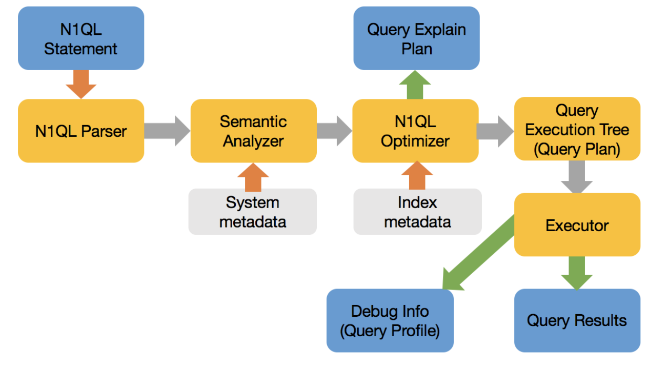
The optimizer, broadly speaking, does the following:
- Rewrite the query to its optimal equivalent form to make the optimization and its choices easier.
- Select the access path for each keyspace (equivalent to tables)
- Select one or more indexes for each keyspace.
- Select the join order for all the joins in the FROM clause. N1QL Optimizer doesn’t reorder the joins yet.
- Select join type (e.g. nested loop or hash join) for each join
- Finally create the query execution tree (plan).
We have described N1QL’s rule-based optimizer in this paper: A Deep Dive Into Couchbase N1QL Query Optimization.
While the discussion in this article is mainly on SELECT statements, the CBO choose query plans for UPDATE, DELETE, MERGE and INSERT (into with SELECT) statements. The challenges, motivation and the solution is equally applicable for all of these DML statements.
N1QL has the following access methods available:
- Value scan
- Key scan
- Index scan
- Covering Index scan
- Primary scan
- Nested loop join
- Hash join
- Unnest scan
Motivation for a Cost Based Optimizer (CBO)

Imagine google maps give you the same route irrespective of the current traffic situation? A cost-based routing takes into consideration the current cost (estimated time based on current traffic flow) and find the fastest route. Similarly, a cost-based optimizer takes into consideration the probable amount of processing (memory, CPU, I/O) for each operation, estimates the cost of alternative routes and selects the query plan (query execution tree) with the least cost. In the example above, the routing algorithm considers the distance, traffic and gave you the three best routes.
For relational systems, CBO was invented in 1970 at IBM, described in this seminal paper. In N1QL’s current rule-based optimizer, planning decisions are independent of the data skew for various access paths and the amount of data that qualifies for the predicates. This results in inconsistent query plan generation and inconsistent performance because the decisions can be less than optimal.
There are many JSON databases: MongoDB, Couchbase, Cosmos DB, CouchDB. Many relational databases support JSON type and accessor functions to index and access data within JSON. Many of them, Couchbase, CosmosDB, MongoDB have a declarative query language for JSON and do access path selection and plan generation. All of them implement rule-based optimizer based on heuristics. We’re yet to see a paper or documentation indicating a cost-based optimizer for any JSON database.
In NoSQL and Hadoop world, there are some examples of a cost-based optimizer.
But, these only handle the basic scalar types, just like relational database optimizer. They do not handle changing types, changing schema, objects, arrays, and array elements — all these are crucial to the success of declarative query language over JSON.
|
1 2 3 4 5 6 7 8 9 10 11 12 13 14 15 16 17 18 19 20 |
Consider the bucket customer: /* Create some indexes */ CREATE PRIMARY index ON customer; CREATE INDEX ix1 ON customer(name, zip, status); CREATE INDEX ix2 ON customer(zip, name, status); CREATE INDEX ix3 ON customer(zip, status, name); CREATE INDEX ix4 ON customer(name, status, zip); CREATE INDEX ix5 ON customer(status, zip, name); CREATE INDEX ix6 ON customer(status, name, zip); CREATE INDEX ix7 ON customer(status); CREATE INDEX ix8 ON customer(name); CREATE INDEX ix9 ON customer(zip); CREATE INDEX ix10 ON customer(status, name); CREATE INDEX ix11 ON customer(status, zip); CREATE INDEX ix12 ON customer(name, zip); |
Example Query:
SELECT * FROM customer WHERE name = “Joe” AND zip = 94587 AND status = “Premium”;
The simple question is:
- All of the indexes above are valid access path to evaluate the query. Which of the several indexes should N1QL use to run the query efficiently?
- The correct answer for this is, it depends. It depends on the cardinality which depends on the statistical distribution of data for each key.
There could be a million people with the name Joe, ten million people in zip code 94587 and only 5 people with Premium status. It could be just a few people with the name Joe or more people with Premium status or fewer customers in the zip 94587. The number of documents qualifying for each filter and the combined statistics affect the decision.
So far, the problems are the same as SQL optimization. Following this approach is safe and sound for collecting statistics, calculating selectivities and coming up with the query plan.
But, JSON is different:
- The data type can change between multiple documents. Zip can be numeric in one document, string in another, the object in the third. How do you collect statistics, store it and use it efficiently?
- It can store complex, a nested structure using arrays and objects. What does it mean to collect statistics on nested structures, arrays, etc?
Scalars: numbers, boolean, string, null, missing. In the document below, a, b, c,d, e are all scalars.
{ “a”: 482, “b”: 2948.284, “c”: “Hello, World”, “d”: null, “e”: missing }
Objects:
- Search for the whole objects
- Search for elements within an objects
- Search for exact value of an attribute within the objects
- Match the elements, arrays, objects anywhere within the hierarchy.
This structure is known only after the user specifies the references to these in the query. If these expressions are in predicates, it would be good to know if they actually exist and then determine their selectivity.
Here are some examples.
Objects:
- Refer to a scalar inside an object. E.g. Name.fname, Name.lname
- Refer to a scalar inside an array of an object. E.g. Billing[*].status
- Nested case of (1), (2) and (3). Using UNNEST operation.
- Refer to an object or an array in the cases (1) through (4).
Arrays:
- Match the full array.
- Match scalar elements of an array with supported types (number, string, etc)
- Match objects within an array.
- Match the elements within an array of an array.
- Match the elements, arrays, objects anywhere within the hierarchy.
LET Expressions:
- Need to get selectivity on the expressions used in the WHERE clause.
UNNEST operation:
- Selectivities on the filters on UNNESTed doc to help pick up the right (array) index.
JOINs: INNER, LEFT OUTER, RIGHT OUTER
- Join selectivities.
- Usually a big problem in RDBMS as well. May not be in v1.
Predicates:
- USE KEYS
- Comparison of scalar values: =, >, <, >=, <=, BETWEEN, IN
- Array predicates: ANY, EVERY, ANY & EVERY, WITHIN
- Subqueries
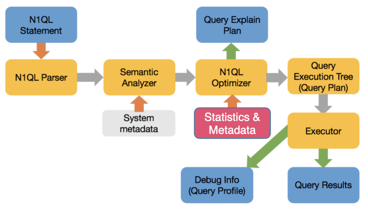
Cost-Based Optimizer for N1QL
The cost-based optimizer will now estimate the cost based on the available statistics on data, index, calculate the cost of each operation and choose the best path.
Challenges to Cost-Based Optimizer for JSON
- Collect statistics on scalars, objects, arrays, array elements — anything on which you can apply a predicate (filter)
- Create the right data structure to store statistics on a field whose type can very from one type to another.
- Create methods to use the statistics to efficiently calculate accurate estimates on complex set of statistics collected above.
- Use appropriate statistics, consider valid access paths, and create a query plan.
- A field can be an integer in one document, string in next, array in another and go missing in yet another. The histograms
Approach to N1QL cost-based optimizer
N1QL optimizer will be responsible for determining the most efficient execution strategy for a query. There are typically a large number of alternative evaluation strategies for a given query. These alternatives may differ significantly in their system resources requirement and/or response time. A cost based query optimizer uses a sophisticated enumeration engine (i.e., an engine that enumerates the search space of access and join plans) to efficiently generate a profusion of alternative query evaluation strategies and a detailed model of execution cost to choose among those alternative strategies.
N1QL Optimizer work can be categorized into these:
- Collect statistics
- Collect statistics on individual fields and create a single histogram for each field (inclusive of all data types that may appear in this field).
- Collect statistics on each available index.
- Query rewrite.
- Basic rule based query rewrite.
- Cardinality estimates
- Use available histogram and index statistics for selectivity estimation.
- Use this selectivity for cardinality estimation
- This is not so straightforward in case of arrays.
- Join ordering.
- CONSIDER a query: a JOIN b JOIN c
- This is same as ( b JOIN a JOIN c), (a JOIN c JOIN b), etc.
- Choosing the right order makes a huge impact on the query.
- The Couchbase 6.5 implementation does not yet do this. This is a well understood problem for which we can borrow solutions from SQL. JSON does not introduce new issues. The ON clause predicates can include array predicates. This is in the roadmap.
- CONSIDER a query: a JOIN b JOIN c
- Join type
- The rule based optimizer used block-nested-loop by default. Need to use directives for forcing hash join. Directive also needs to specify the build/probe side. Both are undesirable.
- CBO should select the join type. If a hash join is chosen, it should automatically choose the build and the probe side. Choosing the best inner/outer keyspace for nested loop is in our roadmap as well.
Statistics Collection for N1QL CBO
Optimizer statistics is an essential part of cost-based optimization. The optimizer calculates costs for various steps of query execution, and the calculation is based on the optimizer’s knowledge on various aspects of the physical entities in the server – known as optimizer statistics.
Handling of mixed types
Unlike relational databases, a field in a JSON document does not have a type, i.e., different types of values can exist in the same field. A distribution therefore needs to handle different types of values. To avoid confusion we put different types of values in different distribution bins. This means we may have partial bins (as last bin) for each type. There are also special handling of the special values MISSING, NULL, TRUE and FALSE. These values (if present) always reside in an overflow bin. N1QL has predefined sorting order for different types and MISSING/NULL/TRUE/FALSE appears at the beginning of the sorted stream.
collection/bucket statistics
For collections or buckets, we gather:
- number of documents in the collection/bucket
- average document size
Index statistics
For a GSI index, we gather:
- number of items in the index
- number of index pages
- resident ratio
- average item size
- average page size
Distribution statistics
For certain fields we also gather distribution statistics, this allows more accurate selectivity estimation for predicates like “c1 = 100”, or “c1 >= 20”, or “c1 < 150”. It also produces more accurate selectivity estimates for join predicates such as “t1.c1 = t2.c2”, assuming distribution statistics exist for both t1.c1 and t2.c2.
Gathering optimizer statistics
While our vision is to have the server automatically update necessary optimizer statistics, for the initial implementation optimizer statistics will be updated via a new UPDATE STATISTICS command.
UPDATE STATISTICS [FOR] <keyspace_reference> (<index_expressions>) [WITH <options>]
<keyspace_reference> is a collection name (we may support bucket as well, it’s undecided at this point).
The command above is for gathering distribution statistics, <index_expressions> is one or more (comma separated) expressions for which distribution statistics is to be collected. We support the same expressions as in CREATE INDEX command, e.g., a field, a nested fields (inside nested objects, e.g. location.lat), an ALL expression for arrays, etc.The WITH clause is optional, if present, it specifies options for the UPDATE STATISTICS command. The options are specified in JSON format similar to how options are specified for other commands like CREATE INDEX or INFER.
Currently the following options are supported in the WITH clause:
- sample_size: for gathering distribution statistics, user can specify a sample size to use. It is an integer number. Note that we also calculate a minimum sample size and we take the larger of the user-specified sample size and calculated minimum sample size.
- resolution: for gathering distribution statistics, indicate how many distribution bins is desired (granularity of the distribution bins). It is specified as a float number, taken as a percentage. E.g., {“resolution”: 1.0} means each distribution bin contains approximately 1 percent of the total documents, i.e., ~100 distribution bins are desired. Default resolution is 1.0 (100 distribution bins). A minimum resolution of 0.02 (5000 distribution bins) and a maximum resolution of 5.0 (20 distribution bins) will be enforced
- update_statistics_timeout: a time-out value (in seconds) can be specified. The UPDATE STATISTICS command times out with an error when the time-out period is reached. If not specified, a default time-out value will be calculated based on the number of samples used.
Handling of mixed types
Unlike relational databases, a field in a JSON document does not have a type, i.e., different types of values can exist in the same field. A distribution therefore needs to handle different types of values. To avoid confusion we put different types of values in different distribution bins. This means we may have partial bins (as last bin) for each type. There are also special handling of the special values MISSING, NULL, TRUE and FALSE. These values (if present) always reside in an overflow bin. N1QL has predefined sorting order for different types and MISSING/NULL/TRUE/FALSE appears at the beginning of the sorted stream.
Boundary bins
Since we only keep the max value for each bin, the min boundary is derived from the max value of the previous bin. This also means that the very first distribution bin does not have a min value. To resolve that, we put a “boundary bin” at the very beginning, this is a special bin with bin size 0, and the only purpose of the bin is to provide a max value, which is the min boundary of the next distribution bin.
Since a distribution may contain multiple types, we separate the types to different distribution bins, and we also put a “boundary bin” for each type, such that we know the minimum value for each type in a distribution.
Example of handling mixed types and boundary bins
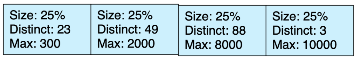
UPDATE STATISTICS for CUSTOMER(quantity);
Histogram: Total number of documents: 5000 with quantity in simple integers.
Predicates:
-
(quantity = 100): Estimate 1%
-
(quantity between 200 and 100) : Estimate 20%
We also use additional techniques like keeping the highest/second-highest, lowest, second lowest values for each bin, keep an overflow bin for values which occur more than 25% of the time to improve this selectivity calculation.
In JSON, quantity can be any of the types: MISSING, null, boolean, integer, string, array and an object. For the sake of simplicity, we show quantity histogram with three types: integers, strings and arrays. This has been extended to include all of the types.
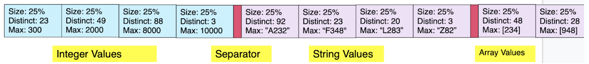
N1QL defines the method by with values of different types can be compared.
- Type order: from lowest to highest
- Missing < null < false < true < numeric < string < array < object
- After we sample the documents, we first group them by types, sort them within the type group and create the mini-histogram for each type.
- We then stitch these mini-histograms into a large histogram with a boundary bin between each type. This helps the optimizer to calculate selectivities efficiently either on a single type or across multiple types.
Examples:
|
1 2 3 4 5 6 7 8 |
WHERE quantity between 100 and 1000; WHERE quantity between 100 and "4829"; WHERE quantity between 100 and [235]; WHERE quantity between 100 and {"val": "2829"}; |
Distribution statistics for simple data types are straight forward. Boolean values will have two overflow bins storing TRUE and FALSE values. Numeric and string values are also easy to handle. An open question remains as to whether we want to limit the size of a string value as a bin boundary, i.e., if a string is very long, do we want to truncate the string before storing as a max value for a distribution bin. Long string values in an overflow bin will not be truncated since that requires an exact match.
The design for how to collect distribution statistics has not been finalized. What we want to do is probably gather distribution statistics on individual elements of the array, since that’s how array index works. We may need to support DISTINCT/ALL variations of the array index by including the same keyword in front of array field specification, which determines whether we remove duplicates from the array before constructing histogram.
Estimating selectivity of an array predicate (ANY predicate) based on such a histogram is a bit challenging. There is no easy way to account for variable lengths of arrays in the collection. In the first release, we’ll just keep an average array size as part of distribution statistics. This assumes some form of uniformity, which is certainly not ideal, but is a good start.
Estimating selectivity of ALL predicate is even trickier, we may need to use some sort of default value for this.
Consider this JSON document in the keyspace
|
1 2 3 4 5 6 7 8 9 10 11 12 |
{ "a": 1, "b": [ 5, 10, 15,20,5,20,10], "c": [ { "x": "hello", "y": true }, { "x": "thanks", "y": false} ] } |
The field “a” is a scalar, b is an array of scalars and c is an array of objects. When is issue a query, you can have predicates on any or all of the fields: a, b, c. So far we’ve discussed the scalars whose type can change. Now let’s discuss array predicates statistics collection and selectivity calculation.
|
1 2 3 4 5 6 7 8 9 10 11 12 13 14 |
Array predicates: FROM k WHERE ANY e IN b SATISFIES e = 10 END FROM k WHERE ANY e in b SATISFIES e > 50 END FROM k WHERE ANY e IN b SATISFIES e BETWEEN 30 and 100 END FROM k UNNEST k.b AS e WHERE e = 10; FROM k UNNEST k.b AS e WHERE e > 10; FROM k WHERE ANY f IN c SATISFIES e.x = “hello” END FROM k WHERE ANY f IN c SATISFIES e.y = true END FROM k UNNEST k.c AS f WHERE f.x = “thanks” |
These are simple predicates on array of scalars and array of objects.This is a generalized implementation where the query can be written to filter elements and value in arrays of arrays, arrays of objects of arrays, etc.
When you have a billion of these documents, you create array indexes to efficiently execute the filter. Now, for the optimizer, it’s important to estimate the number of documents that qualify for a given predicate.
|
1 2 3 4 5 6 7 8 9 |
CREATE INDEX i1 ON k(DISTINCT b); CREATE INDEX I2 ON k (ALL b); CREATE INDEX i3 ON k(DISTINCT array f.x for f IN c) CREATE INDEX i3 ON k(ALL array f.x for f IN c) |
Index i1 with the key DISTINCT b creates an index with only the distinct (unique) elements of b.
Index i2 with the key ALL b creates an index with all the elements of b.
This exists to manage the size of the index, possibility of getting large intermediate results from the index. In both cases, there will be MULTIPLE index entries for EACH element of an array. This is UNLIKE a scalar which has ONLY one entry in the index PER JSON document.
For more on array indexing, see array indexing documentation in Couchbase.
How do you collect statistics on this array or array of objects? The key insight is to collect statistics on EXACTLY the same expression as the expression you’re creating the index on.
In this case, we collect statistics on the following:
|
1 2 3 4 5 6 7 8 |
UPDATE STATISTICS FOR k(DISTINCT b) UPDATE STATISTICS FOR k(ALL b) UPDATE STATISTICS FOR k(DISTINCT array f.x for f IN c) UPDATE STATISTICS FOR k(ALL array f.x for f IN c) |
Now, within the histogram, there can be zero, one or more values originating from the same document. So, calculating the selectivity (estimated percentage of documents qualifying the filter) is not so easy!
Here’s the novel solution to address the issue with arrays:
For normal stats: there’s one index entry per document.
Cardinality becomes a simple: selectivity x table cardinality;
For array stats: There is N index entry per document;
N-> Number of distinct values in the array.
N = 0 to n, n <= ARRAY_LENGTH(a)
This additional statistics has to be collected and stored in the histogram.
Now, when a index is chosen for the evaluation of a particular predicate, index scan will return all of the qualified document keys, which contain duplicates. The query engine will then do a distinct operation to get the unique keys to get the correct (non-duplicate) results. The cost-based optimizer will have to take this into account while calculating the number of documents (not the number of index entries) that’ll qualify the predicate. So, we divide the estimate by the estimate of average array size length.
This cardinality can be used to cost and compare the cost of using the array-index path versus other legal access path to find the best access path.
Object, JSON and binary values
It’s unclear how useful a histogram on an object/JSON value or a binary value will be. It should be rare to see comparisons with such values in the query. We can either handle these exactly like other simple types, i.e., put number of values, number of distinct values, and a max boundary on each distribution bin; or we can simplify and just put the count in the distribution bin without number of distinct and max value. The issue with max value is similar to long strings, where the value can be large, and storing such large values may not be beneficial in the histogram. This remains an open question for now.
Statistics for fields in nested objects
Consider this JSON document in the keyspace:
|
1 2 3 4 5 6 7 8 9 10 11 |
{ "a": 1, "b": {"p": "NY", "q": "212-820-4922", "r": 2848.23}, "c": { "d": 23, "e": { "x": "hello", "y": true , "z": 48} } } |
Following is the dotted expression to access nested objects.
FROM k WHERE b.p = “NY” AND c.e.x = “hello” AND c.e.z = 48;
Since each path is unique, collecting and using the histogram is just like scalar.
UPDATE STATISTICS FOR k(b.p, c.e.x, c.e.z)
Summary
We’ve described how we’ve implemented a cost based optimizer for N1QL (SQL for JSON) and handled the following challenges.
- N1QL CBO can handle flexible JSON schema.
- N1QL CBO can handle scalars, objects, and arrays.
- N1QL CBO can handle stats collection and calculate estimates on any field of any type within JSON.
- All these have improved query plans and therefore improve the performance of the system. It’ll also reduce the TCO by reducing the DBA performance debugging overhead.
- Download Couchbase 6.5 and try it out yourself!
Resources N1QL rule-based Optimizer
The first article describes the Couchbase Optimizer as of 5.0. We added ANSI joins in Couchbase 5.5. The second article includes its description and some of the optimization done for it.
- A Deep Dive Into Couchbase N1QL Query Optimization https://dzone.com/articles/a-deep-dive-into-couchbase-n1ql-query-optimization
- ANSI JOIN Support in N1QL https://dzone.com/articles/ansi-join-support-in-n1ql
- Create the right index, Get the right Performance for the rule-based optimizer.
- Index selection algorithm
References
- Access Path Selection in a Relational Database Management System. https://people.eecs.berkeley.edu/~brewer/cs262/3-selinger79.pdf
- Cost based optimization in DB2 XML. http://www2.hawaii.edu/~lipyeow/pub/ibmsys06-xmlopt.pdf
- Access Path Selection in a Relational Database Management System. https://people.eecs.berkeley.edu/~brewer/cs262/3-selinger79.pdf